Calculating attributable numbers and rates in `cityClimateHealth`
attributable_number.RmdEstimating Attributable numbers (and rates of attributable numbers) are a key way that we can translate relative risks into numbers that are more tangible in public health settings. Below we provide easy functionality to go from our model objects to estimates of attributable numbers and rates.
Setup
The first step of calculating attributable numbers is having a population data estimate.
This varies a lot by place and dataset, so we don’t include
functionality for it (but an example of how this could be done can be
seen in vignette("get_pop_estimates")).
Assume you are starting with a dataset for the entire timeframe that looks like this:
library(data.table)
data("ma_pop_data")
setDT(ma_pop_data)
ma_pop_data
#>               TOWN20 Female_0-17 Female_18-64 Female_65+ Male_0-17 Male_18-64
#>               <char>       <num>        <num>      <num>     <num>      <num>
#>   1:      BARNSTABLE        3899        15017       6014      4499      14035
#>   2:          BOURNE        1891         5751       3212      1489       5302
#>   3:        BREWSTER         634         2518       2007       833       2628
#>   4:         CHATHAM         163         1477       1759       480       1265
#>   5:          DENNIS         573         3792       3133       784       4101
#>  ---
#> 347:   WEST BOYLSTON         619         2021       1107       604       2554
#> 348: WEST BROOKFIELD         343         1162        578       243       1002
#> 349:     WESTMINSTER         847         2371       1131       762       2028
#> 350:      WINCHENDON        1254         3318        711      1031       3134
#> 351:       WORCESTER       18779        67750      15995     21129      69365
#>      Male_65+
#>         <num>
#>   1:     5458
#>   2:     2810
#>   3:     1721
#>   4:     1463
#>   5:     2359
#>  ---
#> 347:      790
#> 348:      495
#> 349:     1081
#> 350:      924
#> 351:    11173
Need to do some transformations:
- pivot longer
- variable clean
Note again, this processing will vary by application so this approach is not prescriptive !
Pivot longer:
ma_pop_data_long <- melt(
  ma_pop_data,
  id.vars = "TOWN20",
  variable.name = "sex_age",
  value.name = "population"
)
Variable clean:
ma_pop_data_long$sex_age <- as.character(ma_pop_data_long$sex_age)
varnames <- strsplit(ma_pop_data_long$sex_age, "_", fixed = T)
varnames <- data.frame(do.call(rbind, varnames))
names(varnames) <- c('sex', 'age_grp')
rr <- which(varnames$sex == 'Female')
varnames$sex[rr] <- 'F'
rr <- which(varnames$sex == 'Male')
varnames$sex[rr] <- 'M'
ma_pop_data_long$sex = varnames$sex
ma_pop_data_long$age_grp = varnames$age_grp
ma_pop_data_long$sex_age <- NULL
ma_pop_data_long
#>                TOWN20 population    sex age_grp
#>                <char>      <num> <char>  <char>
#>    1:      BARNSTABLE       3899      F    0-17
#>    2:          BOURNE       1891      F    0-17
#>    3:        BREWSTER        634      F    0-17
#>    4:         CHATHAM        163      F    0-17
#>    5:          DENNIS        573      F    0-17
#>   ---
#> 2102:   WEST BOYLSTON        790      M     65+
#> 2103: WEST BROOKFIELD        495      M     65+
#> 2104:     WESTMINSTER       1081      M     65+
#> 2105:      WINCHENDON        924      M     65+
#> 2106:       WORCESTER      11173      M     65+
We assume that these properties hold for the entire timeframe of our analysis, but you could also make a version of this dataset with a ‘year’ column.
Now, quickly get a condPois_1stage() and
condPois_2stage() objects to use in testing: exposures
library(data.table)
exposure_columns <- list(
  "date" = "date",
  "exposure" = "tmax_C",
  "geo_unit" = "TOWN20",
  "geo_unit_grp" = "COUNTY20"
)

ma_exposure_matrix <- make_exposure_matrix(
  subset(ma_exposure, COUNTY20 %in% c('MIDDLESEX', 'WORCESTER')),
  exposure_columns,
  time_subset = list(month = 5:9,
                     year = 2013:2015))
#> Warning in make_exposure_matrix(subset(ma_exposure, COUNTY20 %in% c("MIDDLESEX", : check about any NA, some corrections for this later,
#>             but only in certain columns
#> strata dt_by = 'day', setting strata as geo_unit:yr:mn:dow
outcomes
outcome_columns <- list(
  "date" = "date",
  "outcome" = "daily_deaths",
  "factor" = 'age_grp',
  "factor" = 'sex',
  "geo_unit" = "TOWN20",
  "geo_unit_grp" = "COUNTY20"
)

ma_outcomes_tbl <- make_outcome_table(
  subset(ma_deaths,COUNTY20 %in% c('MIDDLESEX', 'WORCESTER')),
  outcome_columns,
  time_subset = list(month = 5:9,
                   year = 2012:2015))
#> > No factors to collapse to, using all data
#> > grp_level == FALSE, so using geo_unit as strata
#> Missing outcome values introduced by xgrid were set to 0;
#>             assumes that every time in the dataset should have an outcome value
#> strata dt_by = 'day', setting strata as geo_unit:yr:mn:dow
models
ma_model <- condPois_2stage(ma_exposure_matrix, ma_outcomes_tbl, verbose = 1, global_cen = 20)
#> -- validation passed
#> -- stage 1
#>
#> crossbasis args:
#>
#> maxlag: 5
#>
#> argvar:
#> List of 2
#>  $ fun  : chr "ns"
#>  $ knots: Named num [1:2] 25.6 31.3
#>   ..- attr(*, "names")= chr [1:2] "50%" "90%"
#>
#> arglag:
#> List of 2
#>  $ fun  : chr "ns"
#>  $ knots: num [1:2] 0.878 2.095
#>
#> strata:
#> ACTON:yr2013:mn05:dow04
#> strata_min: 0
#>
#>
#> -- mixmeta
#> formula: ~ 1 | COUNTY20/TOWN20
#> -- stage 2
Estimating the AN
Ok so now you pass in population.
So now estimate the AN as a full object
Remember that this needs to be compatible for:
single zone
ma model with ma_model$
_ma model with factor ma_model$
0-17> I think you can handle this the same way you did before, with recursion
Now in this second step, you can choose the aggregation level that you want results to.
In this block you need:
what spatial resolution are you summarizing to: ->> ‘geo_unit’, ‘geo_unit_grp’, or ‘all’
are you just getting the impacts that are > then the centering point: ->> lets just assume yes for now, can always go back and change it
ma_AN <- calc_AN(ma_model, ma_outcomes_tbl, ma_pop_data_long,
                 spatial_agg_type = 'TOWN20',
                 spatial_join_col = 'TOWN20',
                 nsim = 100,
                 verbose = 2)
#> -- validation passed
#> -- estimate in each geo_unit
#> 5    10  15  20  25  30  35  40  45  50  55  60  65  70  75  80  85  90  95  100     105     110
#> -- summarize by simulation
#> 5    10  15  20  25  30  35  40  45  50  55  60  65  70  75  80  85  90  95  100
#> -- applying scale of :  1
ma_AN$`_`$rate_table
#>          TOWN20  COUNTY20 population above_MMT mean_annual_attr_rate_est
#>          <char>    <char>      <num>    <lgcl>                     <num>
#>   1:      ACTON MIDDLESEX      23864      TRUE                 2514.2474
#>   2:      ACTON MIDDLESEX      23864     FALSE                 -144.5692
#>   3:  ARLINGTON MIDDLESEX      45906      TRUE                 2610.7698
#>   4:  ARLINGTON MIDDLESEX      45906     FALSE                 -157.1145
#>   5: ASHBURNHAM WORCESTER       6337      TRUE                 1710.1941
#>  ---
#> 224: WINCHESTER MIDDLESEX      22809     FALSE                 -216.4716
#> 225:     WOBURN MIDDLESEX      40992      TRUE                 2522.7483
#> 226:     WOBURN MIDDLESEX      40992     FALSE                 -112.8269
#> 227:  WORCESTER WORCESTER     204191      TRUE                 2284.5032
#> 228:  WORCESTER WORCESTER     204191     FALSE                 -182.3660
#>      mean_annual_attr_rate_lb mean_annual_attr_rate_ub
#>                         <num>                    <num>
#>   1:                1893.4378               3101.63845
#>   2:                -226.5442                -73.77745
#>   3:                2165.2398               3052.66468
#>   4:                -223.0781                -98.95221
#>   5:                1236.4881               2130.54284
#>  ---
#> 224:                -290.5103               -144.57013
#> 225:                1947.1482               3030.16442
#> 226:                -169.2861                -52.43401
#> 227:                1952.5530               2690.48342
#> 228:                -271.4432               -119.06438
ma_AN$`_`$number_table
#>          TOWN20  COUNTY20 population above_MMT mean_annual_attr_num_est
#>          <char>    <char>      <num>    <lgcl>                    <num>
#>   1:      ACTON MIDDLESEX      23864      TRUE                  600.000
#>   2:      ACTON MIDDLESEX      23864     FALSE                  -34.500
#>   3:  ARLINGTON MIDDLESEX      45906      TRUE                 1198.500
#>   4:  ARLINGTON MIDDLESEX      45906     FALSE                  -72.125
#>   5: ASHBURNHAM WORCESTER       6337      TRUE                  108.375
#>  ---
#> 224: WINCHESTER MIDDLESEX      22809     FALSE                  -49.375
#> 225:     WOBURN MIDDLESEX      40992      TRUE                 1034.125
#> 226:     WOBURN MIDDLESEX      40992     FALSE                  -46.250
#> 227:  WORCESTER WORCESTER     204191      TRUE                 4664.750
#> 228:  WORCESTER WORCESTER     204191     FALSE                 -372.375
#>      mean_annual_attr_num_lb mean_annual_attr_num_ub
#>                        <num>                   <num>
#>   1:               451.85000               740.17500
#>   2:               -54.06250               -17.60625
#>   3:               993.97500              1401.35625
#>   4:              -102.40625               -45.42500
#>   5:                78.35625               135.01250
#>  ---
#> 224:               -66.26250               -32.97500
#> 225:               798.17500              1242.12500
#> 226:               -69.39375               -21.49375
#> 227:              3986.93750              5493.72500
#> 228:              -554.26250              -243.11875
you can change spatial_agg_type to be a different
spatial resolution – either whatever the group variable was or “all”
ma_AN <- calc_AN(ma_model, ma_outcomes_tbl, ma_pop_data_long,
                 spatial_agg_type = 'COUNTY20',
                 spatial_join_col = 'TOWN20',
                 nsim = 100,
                 verbose = 2)
#> -- validation passed
#> -- estimate in each geo_unit
#> 5    10  15  20  25  30  35  40  45  50  55  60  65  70  75  80  85  90  95  100     105     110
#> -- summarize by simulation
#> 5    10  15  20  25  30  35  40  45  50  55  60  65  70  75  80  85  90  95  100
#> -- applying scale of :  1
ma_AN$`_`$rate_table
#>     COUNTY20 population above_MMT mean_annual_attr_rate_est
#>       <char>      <num>    <lgcl>                     <num>
#> 1: MIDDLESEX    1623109      TRUE                 2547.2026
#> 2: MIDDLESEX    1623109     FALSE                 -140.2401
#> 3: WORCESTER     858898      TRUE                 2229.6157
#> 4: WORCESTER     858898     FALSE                 -151.1530
#>    mean_annual_attr_rate_lb mean_annual_attr_rate_ub
#>                       <num>                    <num>
#> 1:                2476.7953                2618.7644
#> 2:                -150.7346                -131.6678
#> 3:                2102.1981                2326.5677
#> 4:                -171.5454                -132.5652
ma_AN$`_`$number_table
#>     COUNTY20 population above_MMT mean_annual_attr_num_est
#>       <char>      <num>    <lgcl>                    <num>
#> 1: MIDDLESEX    1623109      TRUE                 41343.88
#> 2: MIDDLESEX    1623109     FALSE                 -2276.25
#> 3: WORCESTER     858898      TRUE                 19150.12
#> 4: WORCESTER     858898     FALSE                 -1298.25
#>    mean_annual_attr_num_lb mean_annual_attr_num_ub
#>                      <num>                   <num>
#> 1:               40201.088               42505.400
#> 2:               -2446.587               -2137.113
#> 3:               18055.738               19982.844
#> 4:               -1473.400               -1138.600
See that the numbers are roughly the same for Suffolk county ? They won’t be exactly the same because of how the averaging works.
Some plot functions exist:
plot(ma_AN, table_type = 'rate', above_MMT = T)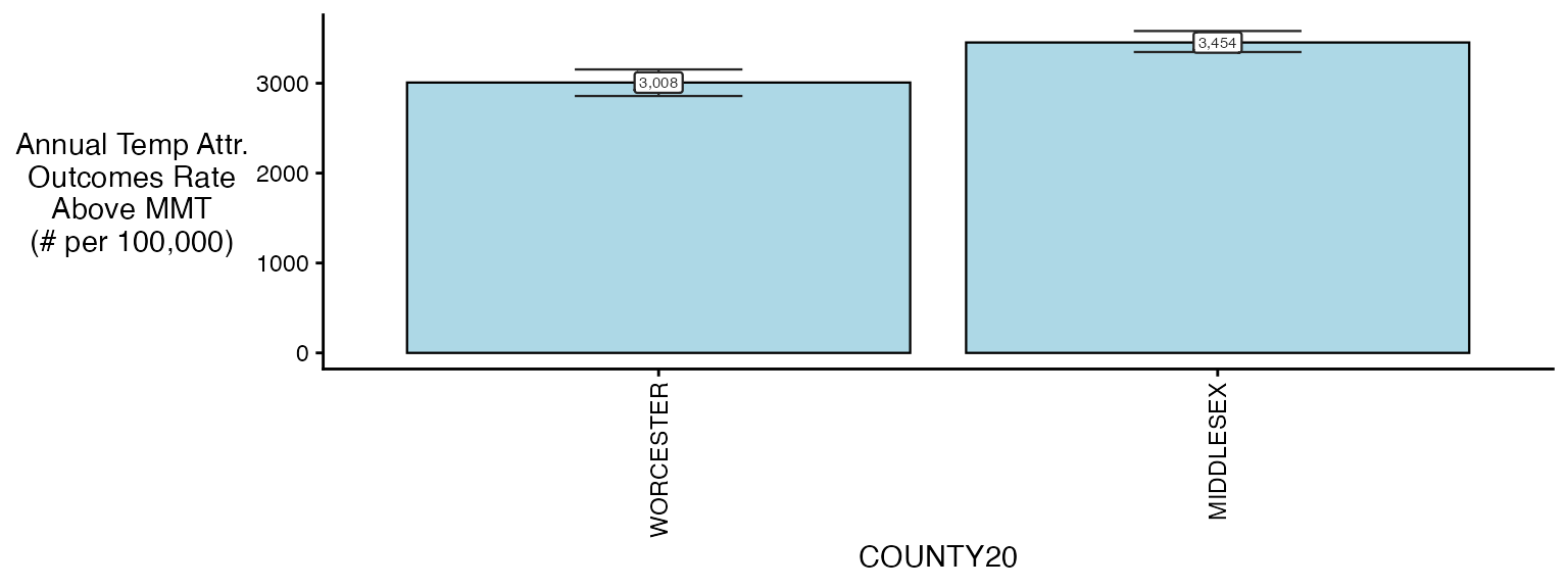
plot(ma_AN, table_type = 'rate', above_MMT = F)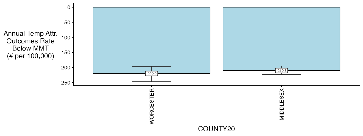
Estimating the AN - single
check of single
# run the model
m2 <- condPois_1stage(exposure_matrix = ma_exposure_matrix,
                  outcomes_tbl = ma_outcomes_tbl,
                  multi_zone = TRUE, global_cen = 15)
#>
#> crossbasis args:
#>
#> maxlag: 5
#>
#> argvar:
#> List of 2
#>  $ fun  : chr "ns"
#>  $ knots: Named num [1:2] 25.3 30.3
#>   ..- attr(*, "names")= chr [1:2] "50%" "90%"
#>
#> arglag:
#> List of 2
#>  $ fun  : chr "ns"
#>  $ knots: num [1:2] 0.878 2.095
#>
#> strata:
#> ACTON:yr2013:mn05:dow04
#> strata_min: 0

ma_AN_s1 <- calc_AN(m2, ma_outcomes_tbl, ma_pop_data_long,
                 spatial_agg_type = 'COUNTY20',
                 spatial_join_col = 'TOWN20',
                 nsim = 100,
                 verbose = 2)
#> -- validation passed
#> -- estimate in each geo_unit
#> 5    10  15  20  25  30  35  40  45  50  55  60  65  70  75  80  85  90  95  100     105     110
#> -- summarize by simulation
#> 5    10  15  20  25  30  35  40  45  50  55  60  65  70  75  80  85  90  95  100
#> -- applying scale of :  1

ma_AN_s1$`_`$rate_table
#>     COUNTY20 population above_MMT mean_annual_attr_rate_est
#>       <char>      <num>    <lgcl>                     <num>
#> 1: MIDDLESEX    1623109      TRUE                3861.70152
#> 2: MIDDLESEX    1623109     FALSE                 -17.17383
#> 3: WORCESTER     858898      TRUE                3644.87401
#> 4: WORCESTER     858898     FALSE                 -23.59128
#>    mean_annual_attr_rate_lb mean_annual_attr_rate_ub
#>                       <num>                    <num>
#> 1:               3841.42447               3881.76372
#> 2:                -17.62513                -16.72562
#> 3:               3599.10097               3682.85582
#> 4:                -24.81450                -22.10172
plot(ma_AN_s1, "num", above_MMT = T)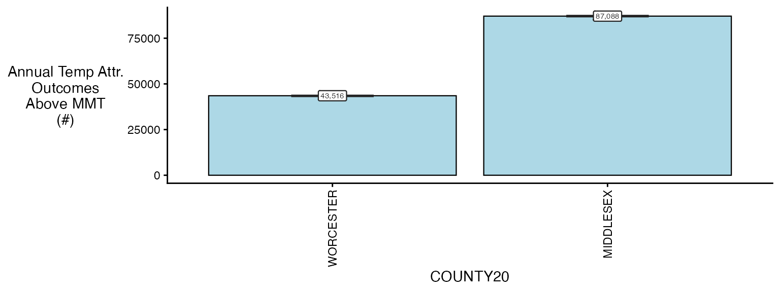
Estimating the AN - with factors
In the case where you have factors, you can easily extend this
ma_outcomes_tbl_fct <- make_outcome_table(
subset(ma_deaths,COUNTY20 %in% c('MIDDLESEX', 'WORCESTER')),
outcome_columns,
time_subset = list(month = 5:9, year = 2012:2015),
collapse_to = 'age_grp')
#> > Factors in data
#> > grp_level == FALSE, so using geo_unit as strata
#> Missing outcome values introduced by xgrid were set to 0;
#> assumes that every time in the dataset should have an outcome value
#> strata dt_by = 'day', setting strata as geo_unit:yr:mn:dow
ma_model_fct <- condPois_2stage(ma_exposure_matrix,
ma_outcomes_tbl_fct,
global_cen = 15,
verbose = 1)
#> < age_grp : 0-17 >
#> -- validation passed
#> -- stage 1
#>
#> crossbasis args:
#>
#> maxlag: 5
#>
#> argvar:
#> List of 2
#> $ fun : chr "ns"
#> $ knots: Named num [1:2] 25.6 31.3
#> ..- attr(*, "names")= chr [1:2] "50%" "90%"
#>
#> arglag:
#> List of 2
#> $ fun : chr "ns"
#> $ knots: num [1:2] 0.878 2.095
#>
#> strata:
#> ACTON:yr2013:mn05:dow04
#> strata_min: 0
#>
#>
#> -- mixmeta
#> formula: ~ 1 | COUNTY20/TOWN20
#> -- stage 2
#>
#> < age_grp : 18-64 >
#> -- validation passed
#> -- stage 1
#>
#> crossbasis args:
#>
#> maxlag: 5
#>
#> argvar:
#> List of 2
#> $ fun : chr "ns"
#> $ knots: Named num [1:2] 25.6 31.3
#> ..- attr(*, "names")= chr [1:2] "50%" "90%"
#>
#> arglag:
#> List of 2
#> $ fun : chr "ns"
#> $ knots: num [1:2] 0.878 2.095
#>
#> strata:
#> ACTON:yr2013:mn05:dow04
#> strata_min: 0
#>
#>
#> -- mixmeta
#> formula: ~ 1 | COUNTY20/TOWN20
#> -- stage 2
#>
#> < age_grp : 65+ >
#> -- validation passed
#> -- stage 1
#>
#> crossbasis args:
#>
#> maxlag: 5
#>
#> argvar:
#> List of 2
#> $ fun : chr "ns"
#> $ knots: Named num [1:2] 25.6 31.3
#> ..- attr(*, "names")= chr [1:2] "50%" "90%"
#>
#> arglag:
#> List of 2
#> $ fun : chr "ns"
#> $ knots: num [1:2] 0.878 2.095
#>
#> strata:
#> ACTON:yr2013:mn05:dow04
#> strata_min: 0
#>
#>
#> -- mixmeta
#> formula: ~ 1 | COUNTY20/TOWN20
#> -- stage 2
ma_AN_fct <- calc_AN(ma_model_fct, ma_outcomes_tbl_fct,
ma_pop_data_long,
spatial_agg_type = 'COUNTY20',
spatial_join_col = 'TOWN20',
nsim = 100,
verbose = 1)
#> -- over-writing `scale` argument with factor scales
#> < age_grp : 0-17 >
#> Warning in calc_AN(model = sub_model, outcomes_tbl = sub_outcomes_tbl, pop_data
#> = sub_pop_data, : some pop data are zero
#> -- validation passed
#> -- estimate in each geo_unit
#> -- summarize by simulation
#> < age_grp : 18-64 >
#> -- validation passed
#> -- estimate in each geo_unit
#> -- summarize by simulation
#> < age_grp : 65+ >
#> -- validation passed
#> -- estimate in each geo_unit
#> -- summarize by simulation
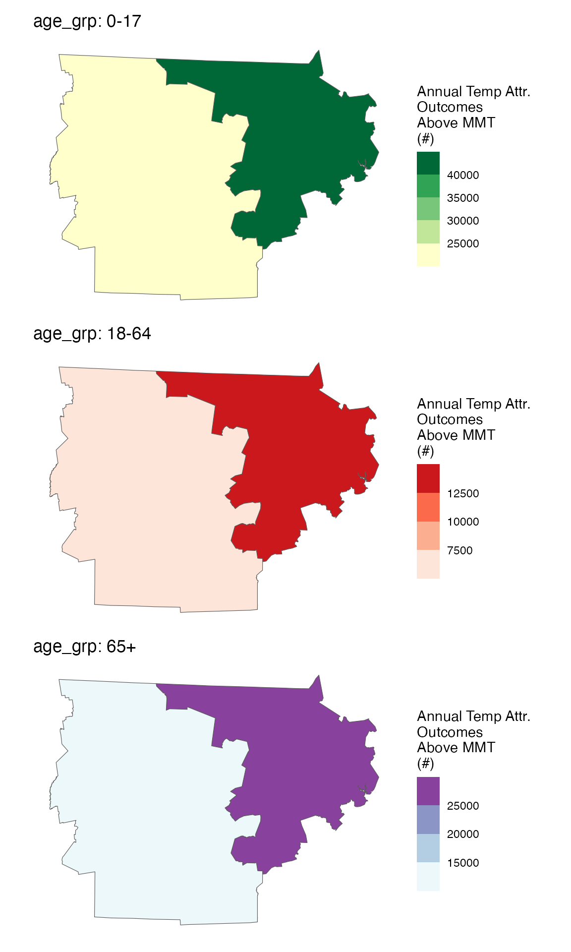
plot(ma_AN_fct, "num", above_MMT = T)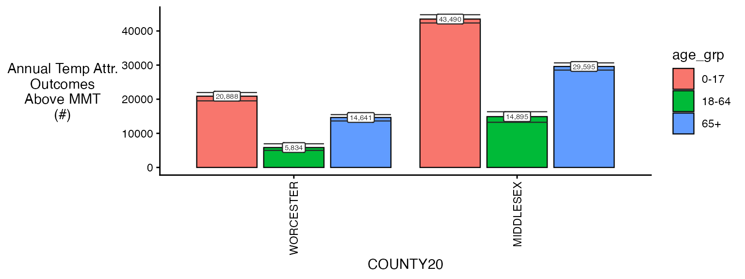
These results are fictional of course but show what kind of outputs can be made easily.
spatial_plot(ma_AN_fct, shp = ma_counties, table_type = "num", above_MMT = T)