Getting started with `cityClimateHealth`
cityClimateHealth.RmdGetting started with cityClimateHealth
Here is code that shows the basic skeleton of how this package works. We can run the model and then calculate attributable numbers easily, and provide a number of outputs.
Run the model
Exposure
First, create the exposure object - you will need to define the
exposure_columns.
library(data.table)

# load a built-in dataset and get a subset
data("ma_exposure")

exposure_sub <-
  subset(ma_exposure,
         COUNTY20 %in% c('MIDDLESEX', 'WORCESTER'))

# define columns of ma_exposure
exposure_columns <- list(
  "date" = "date",
  "exposure" = "tmax_C",
  "geo_unit" = "TOWN20",
  "geo_unit_grp" = "COUNTY20"
)

# create the object
ma_exposure_matrix <- make_exposure_matrix(exposure_sub,
                                           exposure_columns,
                                           time_subset = list(
                                       month = 5:9,
                                       year = 2012:2015
                                     ))
#> Warning in make_exposure_matrix(exposure_sub, exposure_columns, time_subset = list(month = 5:9, : check about any NA, some corrections for this later,
#>             but only in certain columns
#> strata dt_by = 'day', setting strata as geo_unit:yr:mn:dow
And lets preview this
head(ma_exposure_matrix)
#>          date  tmax_C TOWN20  COUNTY20                  strata     match_strata
#>        <IDat>   <num> <char>    <char>                  <char>           <char>
#> 1: 2012-05-01 16.4633  ACTON MIDDLESEX ACTON:yr2012:mn05:dow03 ACTON:2012-05-01
#> 2: 2012-05-02  8.6743  ACTON MIDDLESEX ACTON:yr2012:mn05:dow04 ACTON:2012-05-02
#> 3: 2012-05-03 11.1778  ACTON MIDDLESEX ACTON:yr2012:mn05:dow05 ACTON:2012-05-03
#> 4: 2012-05-04 12.4253  ACTON MIDDLESEX ACTON:yr2012:mn05:dow06 ACTON:2012-05-04
#> 5: 2012-05-05 12.8489  ACTON MIDDLESEX ACTON:yr2012:mn05:dow07 ACTON:2012-05-05
#> 6: 2012-05-06 17.7602  ACTON MIDDLESEX ACTON:yr2012:mn05:dow01 ACTON:2012-05-06
#>    explag1 explag2 explag3 explag4 explag5
#>      <num>   <num>   <num>   <num>   <num>
#> 1: 14.0179 14.1931 12.7975 17.5538 16.2753
#> 2: 16.4633 14.0179 14.1931 12.7975 17.5538
#> 3:  8.6743 16.4633 14.0179 14.1931 12.7975
#> 4: 11.1778  8.6743 16.4633 14.0179 14.1931
#> 5: 12.4253 11.1778  8.6743 16.4633 14.0179
#> 6: 12.8489 12.4253 11.1778  8.6743 16.4633
Outcome
Next, create the outcome object. As seen in other tutorials, you can
collapse_to a factor level and get outputs that way later
on.
# load a built-in dataset, and get a subset, for speed
data("ma_deaths")

deaths_sub <-
  subset(ma_deaths,
        COUNTY20 %in% c('MIDDLESEX', 'WORCESTER'))

# define columns of ma_deaths
outcome_columns <- list(
  "date" = "date",
  "outcome" = "daily_deaths",
  "factor" = 'age_grp',
  "factor" = 'sex',
  "geo_unit" = "TOWN20",
  "geo_unit_grp" = "COUNTY20"
)

# create the object
ma_outcomes_tbl <- make_outcome_table(deaths_sub, outcome_columns,
                                      time_subset = list(
                                       month = 5:9,
                                       year = 2012:2015
                                     ))
#> > No factors to collapse to, using all data
#> > grp_level == FALSE, so using geo_unit as strata
#> Missing outcome values introduced by xgrid were set to 0;
#>             assumes that every time in the dataset should have an outcome value
#> strata dt_by = 'day', setting strata as geo_unit:yr:mn:dow
And lets preview this
head(ma_outcomes_tbl)
#>          date TOWN20  COUNTY20 daily_deaths                  strata
#>        <IDat> <char>    <char>        <int>                  <char>
#> 1: 2012-05-01  ACTON MIDDLESEX           73 ACTON:yr2012:mn05:dow03
#> 2: 2012-05-02  ACTON MIDDLESEX           78 ACTON:yr2012:mn05:dow04
#> 3: 2012-05-03  ACTON MIDDLESEX           78 ACTON:yr2012:mn05:dow05
#> 4: 2012-05-04  ACTON MIDDLESEX           78 ACTON:yr2012:mn05:dow06
#> 5: 2012-05-05  ACTON MIDDLESEX           78 ACTON:yr2012:mn05:dow07
#> 6: 2012-05-06  ACTON MIDDLESEX           72 ACTON:yr2012:mn05:dow01
#>    strata_total     match_strata
#>           <int>           <char>
#> 1:          423 ACTON:2012-05-01
#> 2:          420 ACTON:2012-05-02
#> 3:          414 ACTON:2012-05-03
#> 4:          327 ACTON:2012-05-04
#> 5:          334 ACTON:2012-05-05
#> 6:          334 ACTON:2012-05-06
Run the conditional poisson model
we then run a conditional poisson model.
Cross-basis arguments
There are built-in arguments for argvar and
arglag that you can override if you’d like, but the
defaults are:
-
maxlag: default is 5 (days) -
argvar: default isns()and knots at the 50th and 90th percentile of unit-specific exposure. -
arglag: default islist(fun = 'ns', knots = logknots(maxlag, nk = 2))
You can also affect the global centering point:
- the default behavior is
global_cen = NULL, meaning that the mininum RR will be used - you can override this by setting
global_cen
Model types
Now you have several options for running the conditional poisson model:
| Design | Function | Description |
|---|---|---|
| 1-stage design |
condPois_1stage
|
Produces a single set of beta coefficients across all included spatial
units. If multiple geo_units are present in the input
objects, multi_zone = TRUE must be set. This option does
not use mixmeta or blup.
|
| 2-stage design |
condPois_2stage
|
Estimates beta coefficients for each spatial unit and then uses
mixmeta and blup to obtain more stable
estimates.
|
| Spatial Bayes |
condPois_sb
|
Also estimates beta coefficients for each spatial unit, but applies
Bayesian methods to stabilize estimates by borrowing information from
neighboring spatial units, rather than from the full dataset as in
mixmeta. This approach is especially useful in settings
with small outcome numbers.
|
We show code for each but just run condPois_2stage in
this vignette.
ma_model <- condPois_2stage(ma_exposure_matrix,
                            ma_outcomes_tbl,
                            verbose = 1,
                            global_cen = 15)
#> -- validation passed
#> -- stage 1
#>
#> crossbasis args:
#>
#> maxlag: 5
#>
#> argvar:
#> List of 2
#>  $ fun  : chr "ns"
#>  $ knots: Named num [1:2] 25.7 31.4
#>   ..- attr(*, "names")= chr [1:2] "50%" "90%"
#>
#> arglag:
#> List of 2
#>  $ fun  : chr "ns"
#>  $ knots: num [1:2] 0.878 2.095
#>
#> strata:
#> ACTON:yr2012:mn05:dow03
#> strata_min: 0
#>
#>
#> -- mixmeta
#> formula: ~ 1 | COUNTY20/TOWN20
#> -- stage 2
For condPois_1stage the call would look like this, where
you’d need to add the argument multi_zone = T because there
are multiple geo_units in
ma_exposure_matrix:
ma_model <- condPois_1stage(ma_exposure_matrix, ma_outcomes_tbl,
                            multi_zone = T,
                            global_cen = 15)
See vignette("one_stage_demo") for more details. Note
that forest_plot and spatial_plot are not
implemented for condPois_1stage since you can get all of
that information from the RR plot.
And for condPois_sb, the only additional information
you’d need is a shapefile showing how the geo_units are
arranged, in this case ma_towns (in a test run this code
took 20 minutes to complete for the full MA dataset [with maybe some
additional bugs to work out]):
data("ma_towns")
ma_model <- condPois_sb(ma_exposure_matrix, ma_outcomes_tbl,
                        global_cen = 15, ma_towns)
See vignette("bayesian_demo") for more details.
Plot outputs
And are several plots you can make.
First, a basic RR plot by geo_unit:
plot(ma_model, "CAMBRIDGE")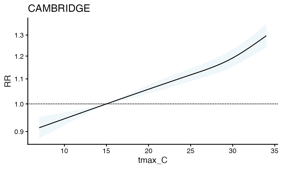
You can also make a forest plot at a specific exposure value
forest_plot(ma_model, exposure_val = 25.1)
#> Warning in forest_plot.condPois_2stage(ma_model, exposure_val = 25.1): plotting
#> by group since n_geos > 20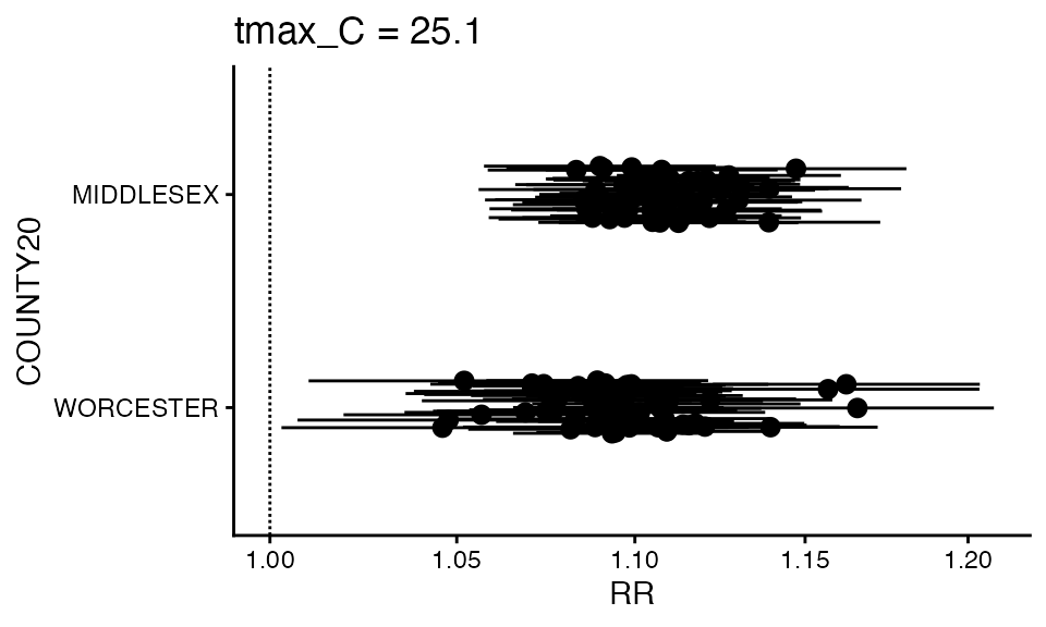
You can also make a spatial plot at a specific exposure value:
spatial_plot(ma_model, shp = ma_towns, exposure_val = 25.1)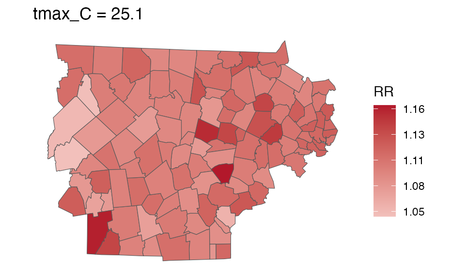
getRR
For your own purposes, each of these objects has a getRR
function
getRR(ma_model)
#>           TOWN20  COUNTY20 tmax_C        RR      RRlb      RRub     model_class
#>           <char>    <char>  <num>     <num>     <num>     <num>          <char>
#>     1:     ACTON MIDDLESEX    7.0 0.9563939 0.9169757 0.9975065 condPois_2stage
#>     2:     ACTON MIDDLESEX    7.1 0.9568875 0.9179730 0.9974517 condPois_2stage
#>     3:     ACTON MIDDLESEX    7.2 0.9573815 0.9189714 0.9973970 condPois_2stage
#>     4:     ACTON MIDDLESEX    7.3 0.9578757 0.9199708 0.9973425 condPois_2stage
#>     5:     ACTON MIDDLESEX    7.4 0.9583704 0.9209713 0.9972882 condPois_2stage
#>    ---
#> 32510: WORCESTER WORCESTER   33.6 1.2260190 1.1798181 1.2740291 condPois_2stage
#> 32511: WORCESTER WORCESTER   33.7 1.2277178 1.1808892 1.2764033 condPois_2stage
#> 32512: WORCESTER WORCESTER   33.8 1.2294189 1.1819524 1.2787916 condPois_2stage
#> 32513: WORCESTER WORCESTER   33.9 1.2311225 1.1830083 1.2811935 condPois_2stage
#> 32514: WORCESTER WORCESTER   34.0 1.2328284 1.1840574 1.2836083 condPois_2stage
Calculate attributable numbers
See more details in vignette("attributable_number"), but
here is a brief demo
Population data
The first step of calculating attributable numbers is having a population data estimate.
This varies a lot by place and dataset, so we don’t include
functionality for it (but an example of how this could be done can be
seen in vignette("get_pop_estimates")).
Assume you are starting with a dataset for the entire timeframe that looks like this:
library(data.table)
data("ma_pop_data")
setDT(ma_pop_data)
ma_pop_data
#>               TOWN20 Female_0-17 Female_18-64 Female_65+ Male_0-17 Male_18-64
#>               <char>       <num>        <num>      <num>     <num>      <num>
#>   1:      BARNSTABLE        3899        15017       6014      4499      14035
#>   2:          BOURNE        1891         5751       3212      1489       5302
#>   3:        BREWSTER         634         2518       2007       833       2628
#>   4:         CHATHAM         163         1477       1759       480       1265
#>   5:          DENNIS         573         3792       3133       784       4101
#>  ---
#> 347:   WEST BOYLSTON         619         2021       1107       604       2554
#> 348: WEST BROOKFIELD         343         1162        578       243       1002
#> 349:     WESTMINSTER         847         2371       1131       762       2028
#> 350:      WINCHENDON        1254         3318        711      1031       3134
#> 351:       WORCESTER       18779        67750      15995     21129      69365
#>      Male_65+
#>         <num>
#>   1:     5458
#>   2:     2810
#>   3:     1721
#>   4:     1463
#>   5:     2359
#>  ---
#> 347:      790
#> 348:      495
#> 349:     1081
#> 350:      924
#> 351:    11173
Need to do some transformations:
- pivot longer
- variable clean
Note again, this processing will vary by application so this approach is not prescriptive !
Pivot longer:
ma_pop_data_long <- melt(
  ma_pop_data,
  id.vars = "TOWN20",
  variable.name = "sex_age",
  value.name = "population"
)
Variable clean:
ma_pop_data_long$sex_age <- as.character(ma_pop_data_long$sex_age)
varnames <- strsplit(ma_pop_data_long$sex_age, "_", fixed = T)
varnames <- data.frame(do.call(rbind, varnames))
names(varnames) <- c('sex', 'age_grp')
rr <- which(varnames$sex == 'Female')
varnames$sex[rr] <- 'F'
rr <- which(varnames$sex == 'Male')
varnames$sex[rr] <- 'M'
ma_pop_data_long$sex = varnames$sex
ma_pop_data_long$age_grp = varnames$age_grp
ma_pop_data_long$sex_age <- NULL
Lets look at it:
ma_pop_data_long
#>                TOWN20 population    sex age_grp
#>                <char>      <num> <char>  <char>
#>    1:      BARNSTABLE       3899      F    0-17
#>    2:          BOURNE       1891      F    0-17
#>    3:        BREWSTER        634      F    0-17
#>    4:         CHATHAM        163      F    0-17
#>    5:          DENNIS        573      F    0-17
#>   ---
#> 2102:   WEST BOYLSTON        790      M     65+
#> 2103: WEST BROOKFIELD        495      M     65+
#> 2104:     WESTMINSTER       1081      M     65+
#> 2105:      WINCHENDON        924      M     65+
#> 2106:       WORCESTER      11173      M     65+
We assume that these properties hold for the entire timeframe of our analysis, but you could also make a version of this dataset with a ‘year’ column.
Calculate AN
Now, you can easily calculate attributrable numbers (and rates) using
calcAN().
There are two new inputs that this function needs, in addition to population data:
-
spatial_agg_type- what spatial resolution are you summarizing to: ‘geo_unit’, ‘geo_unit_grp’, or ‘all’ -
spatial_join_col- which columns inma_outcomes_tblare you joiningma_pop_data_longby
ma_AN <- calc_AN(ma_model, ma_outcomes_tbl, ma_pop_data_long,
                 spatial_agg_type = 'TOWN20', spatial_join_col = 'TOWN20')
From this you get a rate_table :
ma_AN$`_`$rate_table
#>          TOWN20  COUNTY20 population above_MMT mean_annual_attr_rate_est
#>          <char>    <char>      <num>    <lgcl>                     <num>
#>   1:      ACTON MIDDLESEX      23864      TRUE                5191.92089
#>   2:      ACTON MIDDLESEX      23864     FALSE                 -30.38049
#>   3:  ARLINGTON MIDDLESEX      45906      TRUE                5854.89914
#>   4:  ARLINGTON MIDDLESEX      45906     FALSE                 -43.02270
#>   5: ASHBURNHAM WORCESTER       6337      TRUE                4025.95866
#>  ---
#> 224: WINCHESTER MIDDLESEX      22809     FALSE                 -51.51475
#> 225:     WOBURN MIDDLESEX      40992      TRUE                5067.45219
#> 226:     WOBURN MIDDLESEX      40992     FALSE                 -21.95550
#> 227:  WORCESTER WORCESTER     204191      TRUE                5012.28017
#> 228:  WORCESTER WORCESTER     204191     FALSE                 -36.36301
#>      mean_annual_attr_rate_lb mean_annual_attr_rate_ub
#>                         <num>                    <num>
#>   1:               4087.64247              6439.354257
#>   2:                -61.80858                -1.047603
#>   3:               4769.62434              6928.751144
#>   4:                -67.01194               -20.408552
#>   5:               3161.88654              4983.036137
#>  ---
#> 224:                -77.82016               -26.826034
#> 225:               3953.21038              6227.953015
#> 226:                -38.74232                -4.269126
#> 227:               4032.24799              5995.700716
#> 228:                -60.13365               -15.512437
and a number_table:
ma_AN$`_`$number_table
#>          TOWN20  COUNTY20 population above_MMT mean_annual_attr_num_est
#>          <char>    <char>      <num>    <lgcl>                    <num>
#>   1:      ACTON MIDDLESEX      23864      TRUE                 1239.000
#>   2:      ACTON MIDDLESEX      23864     FALSE                   -7.250
#>   3:  ARLINGTON MIDDLESEX      45906      TRUE                 2687.750
#>   4:  ARLINGTON MIDDLESEX      45906     FALSE                  -19.750
#>   5: ASHBURNHAM WORCESTER       6337      TRUE                  255.125
#>  ---
#> 224: WINCHESTER MIDDLESEX      22809     FALSE                  -11.750
#> 225:     WOBURN MIDDLESEX      40992      TRUE                 2077.250
#> 226:     WOBURN MIDDLESEX      40992     FALSE                   -9.000
#> 227:  WORCESTER WORCESTER     204191      TRUE                10234.625
#> 228:  WORCESTER WORCESTER     204191     FALSE                  -74.250
#>      mean_annual_attr_num_lb mean_annual_attr_num_ub
#>                        <num>                   <num>
#>   1:               975.47500              1536.68750
#>   2:               -14.75000                -0.25000
#>   3:              2189.54375              3180.71250
#>   4:               -30.76250                -9.36875
#>   5:               200.36875               315.77500
#>  ---
#> 224:               -17.75000                -6.11875
#> 225:              1620.50000              2552.96250
#> 226:               -15.88125                -1.75000
#> 227:              8233.48750             12242.68125
#> 228:              -122.78750               -31.67500
And you can plot either one
plot(ma_AN, "num", above_MMT = T)
#> Warning in plot.calcAN(ma_AN, "num", above_MMT = T): plot elements > 20,
#> subsetting to top 20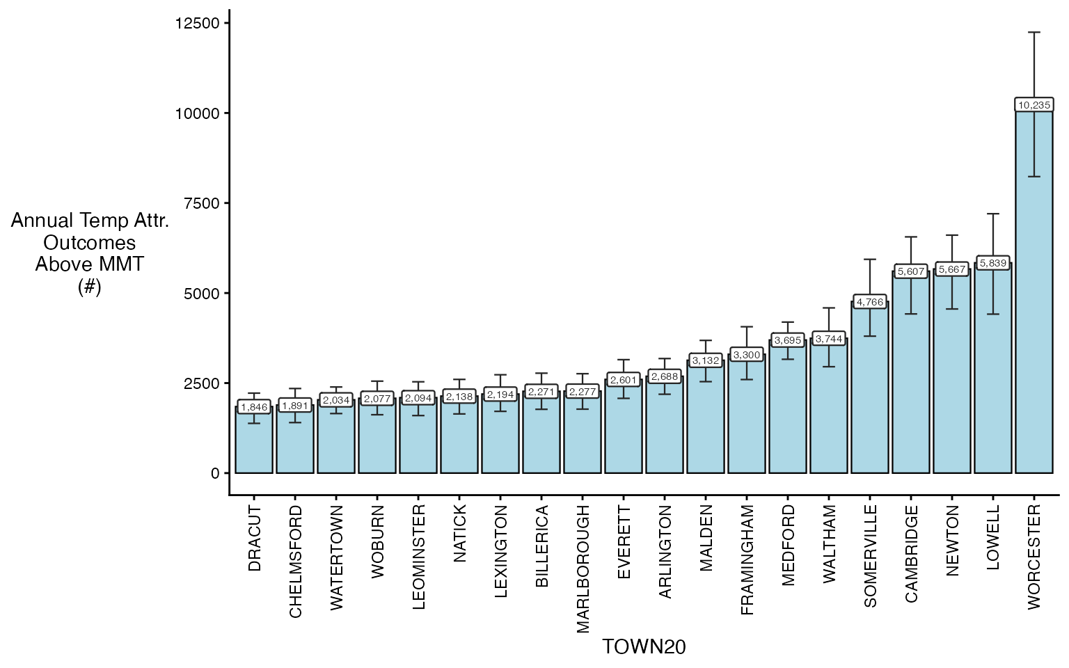
You can also plot spatially
spatial_plot(ma_AN, shp = ma_towns, table_type = "num", above_MMT = T)
Running with factors
Very often, we also get asked to run these results, with differences by both modifiable and non-modifiable factors:
- age group
- sex
- the prevalence of air conditioning in a certain town
We can easily do this, by using the collapse_to
argument:
ma_outcomes_tbl_fct <- make_outcome_table(
  deaths_sub, outcome_columns,
  time_subset = list(
       month = 5:9,
       year = 2012:2015
     ),
  collapse_to = 'age_grp')
#> > Factors in data
#> > grp_level == FALSE, so using geo_unit as strata
#> Missing outcome values introduced by xgrid were set to 0;
#>             assumes that every time in the dataset should have an outcome value
#> strata dt_by = 'day', setting strata as geo_unit:yr:mn:dow
Lets look at the result:
head(ma_outcomes_tbl_fct)
#>          date TOWN20  COUNTY20 age_grp daily_deaths                  strata
#>        <IDat> <char>    <char>  <char>        <int>                  <char>
#> 1: 2012-05-01  ACTON MIDDLESEX    0-17           25 ACTON:yr2012:mn05:dow03
#> 2: 2012-05-01  ACTON MIDDLESEX   18-64           24 ACTON:yr2012:mn05:dow03
#> 3: 2012-05-01  ACTON MIDDLESEX     65+           24 ACTON:yr2012:mn05:dow03
#> 4: 2012-05-02  ACTON MIDDLESEX    0-17           26 ACTON:yr2012:mn05:dow04
#> 5: 2012-05-02  ACTON MIDDLESEX   18-64           26 ACTON:yr2012:mn05:dow04
#> 6: 2012-05-02  ACTON MIDDLESEX     65+           26 ACTON:yr2012:mn05:dow04
#>    strata_total     match_strata
#>           <int>           <char>
#> 1:          423 ACTON:2012-05-01
#> 2:          423 ACTON:2012-05-01
#> 3:          423 ACTON:2012-05-01
#> 4:          420 ACTON:2012-05-02
#> 5:          420 ACTON:2012-05-02
#> 6:          420 ACTON:2012-05-02
Now, all of our other functions can stay the same:
Running the model (adding the verbose argument so you
can follow along)
ma_model_fct <- condPois_2stage(ma_exposure_matrix, ma_outcomes_tbl_fct,
                                verbose = 1, global_cen = 15)
#> < age_grp : 0-17 >
#> -- validation passed
#> -- stage 1
#>
#> crossbasis args:
#>
#> maxlag: 5
#>
#> argvar:
#> List of 2
#>  $ fun  : chr "ns"
#>  $ knots: Named num [1:2] 25.7 31.4
#>   ..- attr(*, "names")= chr [1:2] "50%" "90%"
#>
#> arglag:
#> List of 2
#>  $ fun  : chr "ns"
#>  $ knots: num [1:2] 0.878 2.095
#>
#> strata:
#> ACTON:yr2012:mn05:dow03
#> strata_min: 0
#>
#>
#> -- mixmeta
#> formula: ~ 1 | COUNTY20/TOWN20
#> -- stage 2
#>
#> < age_grp : 18-64 >
#> -- validation passed
#> -- stage 1
#>
#> crossbasis args:
#>
#> maxlag: 5
#>
#> argvar:
#> List of 2
#>  $ fun  : chr "ns"
#>  $ knots: Named num [1:2] 25.7 31.4
#>   ..- attr(*, "names")= chr [1:2] "50%" "90%"
#>
#> arglag:
#> List of 2
#>  $ fun  : chr "ns"
#>  $ knots: num [1:2] 0.878 2.095
#>
#> strata:
#> ACTON:yr2012:mn05:dow03
#> strata_min: 0
#>
#>
#> -- mixmeta
#> formula: ~ 1 | COUNTY20/TOWN20
#> -- stage 2
#>
#> < age_grp : 65+ >
#> -- validation passed
#> -- stage 1
#>
#> crossbasis args:
#>
#> maxlag: 5
#>
#> argvar:
#> List of 2
#>  $ fun  : chr "ns"
#>  $ knots: Named num [1:2] 25.7 31.4
#>   ..- attr(*, "names")= chr [1:2] "50%" "90%"
#>
#> arglag:
#> List of 2
#>  $ fun  : chr "ns"
#>  $ knots: num [1:2] 0.878 2.095
#>
#> strata:
#> ACTON:yr2012:mn05:dow03
#> strata_min: 0
#>
#>
#> -- mixmeta
#> formula: ~ 1 | COUNTY20/TOWN20
#> -- stage 2
And plotting the output
plot(ma_model_fct, "CAMBRIDGE")
forest_plot(ma_model_fct, exposure_val = 25.1)
#> Warning in forest_plot.condPois_2stage_list(ma_model_fct, exposure_val = 25.1):
#> plotting by group since n_geos > 20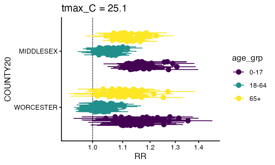
You can also make a spatial plot at a specific exposure value:
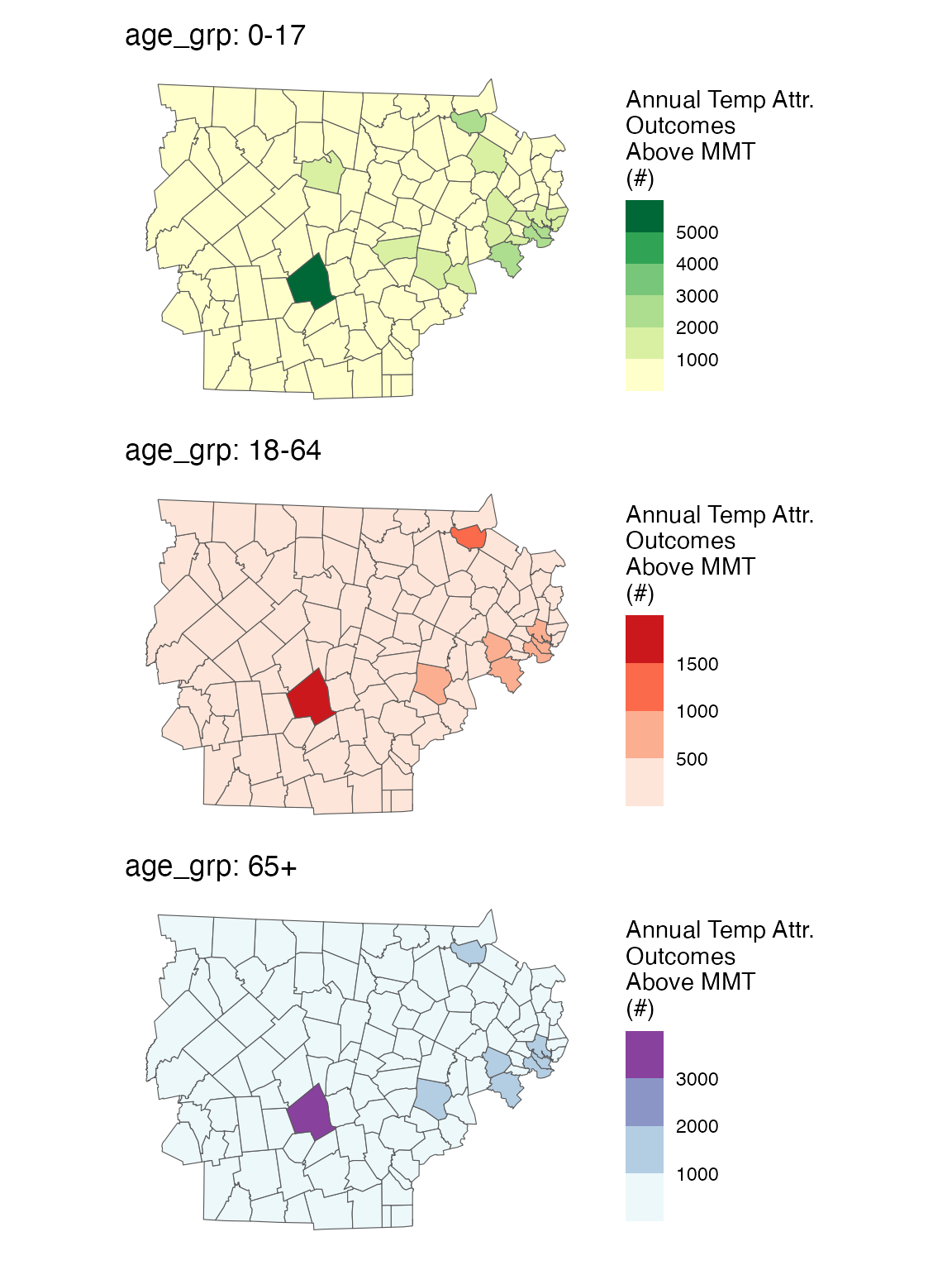
spatial_plot(ma_model_fct, shp = ma_towns, exposure_val = 25.1)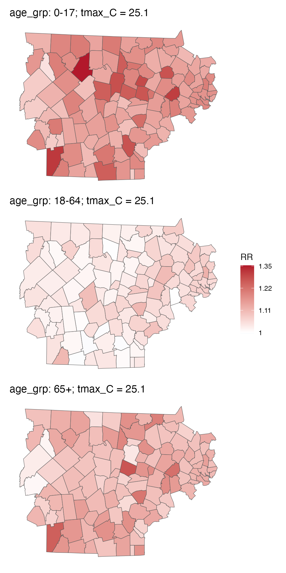
You can also getRR:
getRR(ma_model_fct)
#>           TOWN20  COUNTY20 tmax_C        RR      RRlb      RRub age_grp
#>           <char>    <char>  <num>     <num>     <num>     <num>  <char>
#>     1:     ACTON MIDDLESEX    7.0 0.9414289 0.8898588 0.9959876    0-17
#>     2:     ACTON MIDDLESEX    7.1 0.9420825 0.8911541 0.9959214    0-17
#>     3:     ACTON MIDDLESEX    7.2 0.9427367 0.8924513 0.9958554    0-17
#>     4:     ACTON MIDDLESEX    7.3 0.9433914 0.8937504 0.9957895    0-17
#>     5:     ACTON MIDDLESEX    7.4 0.9440467 0.8950514 0.9957240    0-17
#>    ---
#> 97538: WORCESTER WORCESTER   33.6 1.2231257 1.1800147 1.2678116     65+
#> 97539: WORCESTER WORCESTER   33.7 1.2246071 1.1807440 1.2700996     65+
#> 97540: WORCESTER WORCESTER   33.8 1.2260900 1.1814480 1.2724190     65+
#> 97541: WORCESTER WORCESTER   33.9 1.2275747 1.1821281 1.2747685     65+
#> 97542: WORCESTER WORCESTER   34.0 1.2290611 1.1827859 1.2771468     65+
#>                 model_class
#>                      <char>
#>     1: condPois_2stage_list
#>     2: condPois_2stage_list
#>     3: condPois_2stage_list
#>     4: condPois_2stage_list
#>     5: condPois_2stage_list
#>    ---
#> 97538: condPois_2stage_list
#> 97539: condPois_2stage_list
#> 97540: condPois_2stage_list
#> 97541: condPois_2stage_list
#> 97542: condPois_2stage_list
And finally, you can calcAN, note that both
ma_outcomes_tbl_fct and ma_model_fct need to
have factors, again adding the verbose so you can see the progress
ma_AN_fct <- calc_AN(ma_model_fct,
                     ma_outcomes_tbl_fct,
                     ma_pop_data_long,
                 spatial_agg_type = 'TOWN20', spatial_join_col = 'TOWN20',
                 verbose = 1)
#> -- over-writing `scale` argument with factor scales
#> < age_grp : 0-17 >
#> Warning in calc_AN(model = sub_model, outcomes_tbl = sub_outcomes_tbl, pop_data
#> = sub_pop_data, : some pop data are zero
#> -- validation passed
#> -- estimate in each geo_unit
#> -- summarize by simulation
#> < age_grp : 18-64 >
#> -- validation passed
#> -- estimate in each geo_unit
#> -- summarize by simulation
#> < age_grp : 65+ >
#> -- validation passed
#> -- estimate in each geo_unit
#> -- summarize by simulation
And you can plot either one – some empty bars not because there are no adults there but because this takes the top 20 in each bin, which don’t have to overlap. Probably a better way to do this in the future but fine for diagnostics.
plot(ma_AN_fct, "num", above_MMT = T)
#> Warning in plot.calcAN_list(ma_AN_fct, "num", above_MMT = T): plot elements >
#> 20, subsetting to top 20
#> Warning in plot.calcAN_list(ma_AN_fct, "num", above_MMT = T): plot elements >
#> 20, subsetting to top 20
#> Warning in plot.calcAN_list(ma_AN_fct, "num", above_MMT = T): plot elements >
#> 20, subsetting to top 20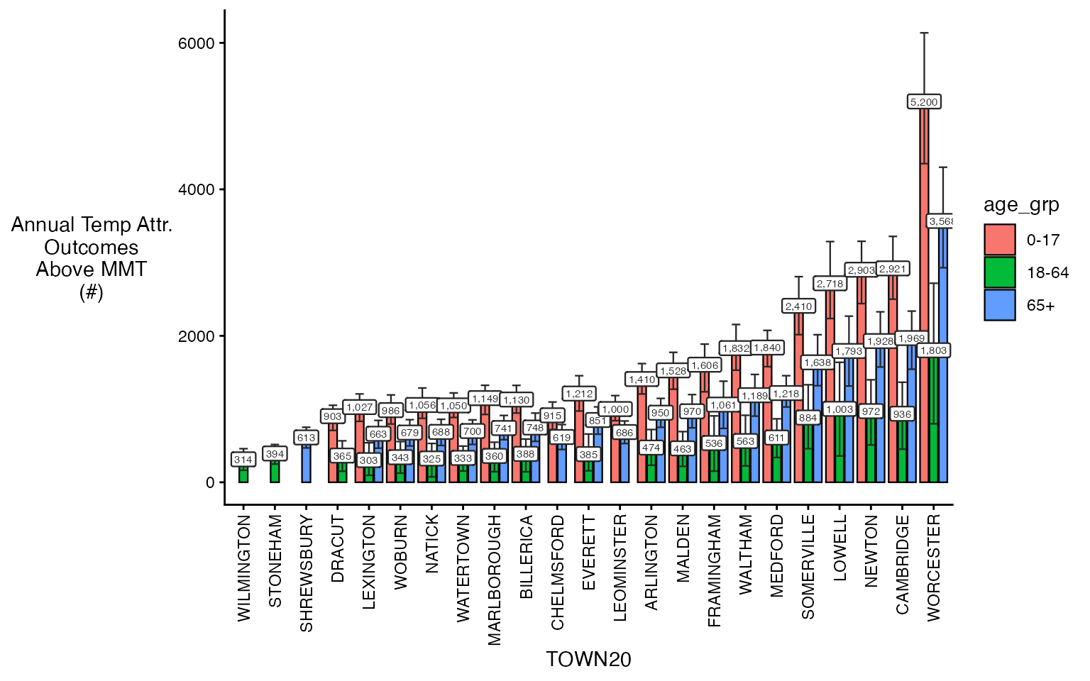
You can also make use of some additional arguments to get plot
subsets, including spatial_sub and
ordered_levels.
plot(ma_AN_fct, 'rate', above_MMT = T,
     spatial_sub = c('BOSTON', 'CAMBRIDGE'),
     ordered_levels = c("0-17", "18-64", "65+"))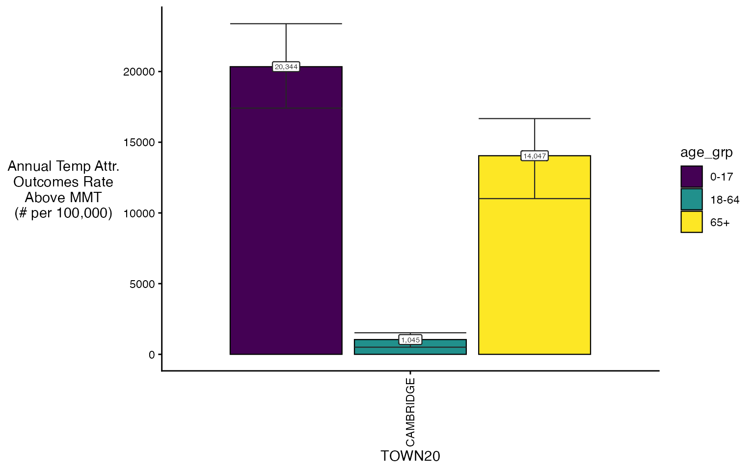
You can also plot spatially
spatial_plot(ma_AN_fct, shp = ma_towns, table_type = "num", above_MMT = T)