One set of Heat-Health Associations for a single or multiple zones using `cityClimateHealth`
one_stage_demo.RmdLet’s use built-in functions to examine a single set of beta
coefficients for heat-health relationships in a single or multiple
geographic unit. We’ll start with a review of DLNM, and then show how
its implemented in cityClimateHealth for both the single
and multi-zone cases.
For testing purposes, start with your largest geographic unit!
Exposure data
First let’s make the exposure matrix for this single zone. There is a
simulated exposure dataset included in the package called
ma_exposure, which lists daily maximum
temperatures each day in each town.
boston_exposure <- subset(ma_exposure, TOWN20 == 'BOSTON')
head(boston_exposure)
#>              date  tmax_C TOWN20 COUNTY20
#> 137783 2010-01-01 -0.3825 BOSTON  SUFFOLK
#> 137784 2010-01-02  1.4337 BOSTON  SUFFOLK
#> 137785 2010-01-03 -1.4163 BOSTON  SUFFOLK
#> 137786 2010-01-04 -0.4483 BOSTON  SUFFOLK
#> 137787 2010-01-05  0.6565 BOSTON  SUFFOLK
#> 137788 2010-01-06  1.2098 BOSTON  SUFFOLK
Notice how this dataset contains temperature for the whole year. This is a good starting place.
Also notice that these data are messy, as is common in environmental data, there are both NA values and days where there are no measurements:
# Sept 17 2010 has NA data
boston_exposure[255:260,]
#>              date  tmax_C TOWN20 COUNTY20
#> 138037 2010-09-16 19.3761 BOSTON  SUFFOLK
#> 138038 2010-09-17      NA BOSTON  SUFFOLK
#> 138039 2010-09-18 19.0647 BOSTON  SUFFOLK
#> 138040 2010-09-19 19.6014 BOSTON  SUFFOLK
#> 138041 2010-09-20 23.6339 BOSTON  SUFFOLK
#> 138042 2010-09-21 20.8122 BOSTON  SUFFOLK

# July 13 2010 is missing
boston_exposure[190:195,]
#>              date  tmax_C TOWN20 COUNTY20
#> 137972 2010-07-12 31.7248 BOSTON  SUFFOLK
#> 137973 2010-07-14 31.9374 BOSTON  SUFFOLK
#> 137974 2010-07-15 23.7004 BOSTON  SUFFOLK
#> 137975 2010-07-16 28.7843 BOSTON  SUFFOLK
#> 137976 2010-07-17 33.3453 BOSTON  SUFFOLK
#> 137977 2010-07-18 33.1227 BOSTON  SUFFOLK
In the next step we’ll introduce a function which (a) cleans the data and (b) subsets to just warm season months (which in Boston is May through September). Its good to keep the full temperature range before this point so we can use extra data around the cutoffs to make sure the temperature matrix is full.
First, define the column mapping. The main geographic unit of
analysis (the geo_unit) is called TOWN20,
however we may also want to aggregate in some later steps to the group
level, so the grouping variable (geo_unit_grp) is called
COUNTY20. Providing a named list in this way avoids having
to rename columns throughout the process.
exposure_columns <- list(
  "date" = "date",
  "exposure" = "tmax_C",
  "geo_unit" = "TOWN20",
  "geo_unit_grp" = "COUNTY20"
)
Next pass in your full temperature time-series in this step.
boston_exposure_mat <- make_exposure_matrix(boston_exposure,
                                            exposure_columns,
                                            time_subset = list(month = 5:9))
#> Warning in make_exposure_matrix(boston_exposure, exposure_columns, time_subset = list(month = 5:9)): check about any NA, some corrections for this later,
#>             but only in certain columns
#> strata dt_by = 'day', setting strata as geo_unit:yr:mn:dow
head(boston_exposure_mat)
#>          date  tmax_C TOWN20 COUNTY20                   strata
#>        <IDat>   <num> <char>   <char>                   <char>
#> 1: 2010-05-01 23.1386 BOSTON  SUFFOLK BOSTON:yr2010:mn05:dow07
#> 2: 2010-05-02 26.1014 BOSTON  SUFFOLK BOSTON:yr2010:mn05:dow01
#> 3: 2010-05-03 31.5648 BOSTON  SUFFOLK BOSTON:yr2010:mn05:dow02
#> 4: 2010-05-04 27.7814 BOSTON  SUFFOLK BOSTON:yr2010:mn05:dow03
#> 5: 2010-05-05 26.2820 BOSTON  SUFFOLK BOSTON:yr2010:mn05:dow04
#> 6: 2010-05-06 25.8546 BOSTON  SUFFOLK BOSTON:yr2010:mn05:dow05
#>         match_strata  explag1  explag2  explag3  explag4  explag5
#>               <char>    <num>    <num>    <num>    <num>    <num>
#> 1: BOSTON:2010-05-01 15.73815  8.33770 10.85230 16.44320 18.74090
#> 2: BOSTON:2010-05-02 23.13860 15.73815  8.33770 10.85230 16.44320
#> 3: BOSTON:2010-05-03 26.10140 23.13860 15.73815  8.33770 10.85230
#> 4: BOSTON:2010-05-04 31.56480 26.10140 23.13860 15.73815  8.33770
#> 5: BOSTON:2010-05-05 27.78140 31.56480 26.10140 23.13860 15.73815
#> 6: BOSTON:2010-05-06 26.28200 27.78140 31.56480 26.10140 23.13860
You can check that the two problems we saw before – missing data and NA data – are gone now
# Sept 17 2010 now has NA data
boston_exposure_mat[138:142,]
#>          date  tmax_C TOWN20 COUNTY20                   strata
#>        <IDat>   <num> <char>   <char>                   <char>
#> 1: 2010-09-15 22.5722 BOSTON  SUFFOLK BOSTON:yr2010:mn09:dow04
#> 2: 2010-09-16 19.3761 BOSTON  SUFFOLK BOSTON:yr2010:mn09:dow05
#> 3: 2010-09-17 19.2204 BOSTON  SUFFOLK BOSTON:yr2010:mn09:dow06
#> 4: 2010-09-18 19.0647 BOSTON  SUFFOLK BOSTON:yr2010:mn09:dow07
#> 5: 2010-09-19 19.6014 BOSTON  SUFFOLK BOSTON:yr2010:mn09:dow01
#>         match_strata explag1 explag2 explag3 explag4 explag5
#>               <char>   <num>   <num>   <num>   <num>   <num>
#> 1: BOSTON:2010-09-15 19.8015 18.5063 22.8082 20.9759 22.0336
#> 2: BOSTON:2010-09-16 22.5722 19.8015 18.5063 22.8082 20.9759
#> 3: BOSTON:2010-09-17 19.3761 22.5722 19.8015 18.5063 22.8082
#> 4: BOSTON:2010-09-18 19.2204 19.3761 22.5722 19.8015 18.5063
#> 5: BOSTON:2010-09-19 19.0647 19.2204 19.3761 22.5722 19.8015

# July 13 2010 is now not missing
boston_exposure_mat[72:77,]
#>          date  tmax_C TOWN20 COUNTY20                   strata
#>        <IDat>   <num> <char>   <char>                   <char>
#> 1: 2010-07-11 29.1988 BOSTON  SUFFOLK BOSTON:yr2010:mn07:dow01
#> 2: 2010-07-12 31.7248 BOSTON  SUFFOLK BOSTON:yr2010:mn07:dow02
#> 3: 2010-07-13 31.8311 BOSTON  SUFFOLK BOSTON:yr2010:mn07:dow03
#> 4: 2010-07-14 31.9374 BOSTON  SUFFOLK BOSTON:yr2010:mn07:dow04
#> 5: 2010-07-15 23.7004 BOSTON  SUFFOLK BOSTON:yr2010:mn07:dow05
#> 6: 2010-07-16 28.7843 BOSTON  SUFFOLK BOSTON:yr2010:mn07:dow06
#>         match_strata explag1 explag2 explag3 explag4 explag5
#>               <char>   <num>   <num>   <num>   <num>   <num>
#> 1: BOSTON:2010-07-11 33.0867 32.8450 34.5714 37.1773 36.2254
#> 2: BOSTON:2010-07-12 29.1988 33.0867 32.8450 34.5714 37.1773
#> 3: BOSTON:2010-07-13 31.7248 29.1988 33.0867 32.8450 34.5714
#> 4: BOSTON:2010-07-14 31.8311 31.7248 29.1988 33.0867 32.8450
#> 5: BOSTON:2010-07-15 31.9374 31.8311 31.7248 29.1988 33.0867
#> 6: BOSTON:2010-07-16 23.7004 31.9374 31.8311 31.7248 29.1988
Its probably a good idea to see if there is any systematic bias in the missingness (i.e., are the data “missing at random”) but for the purposes of this tutorial we’ll assume that they are (which is true since these are simulated data!).
It may also be a good idea to check that the exposure values generally look like you expect them to look (e.g., with some summary statistics), just to make sure you don’t need to do anys additional pre-processing (e.g., if there are location-specific wildly high or low temperatures, this script as is will not catch those).
summary(boston_exposure_mat$tmax_C)
#>    Min. 1st Qu.  Median    Mean 3rd Qu.    Max.
#>   6.762  22.059  26.184  25.385  29.225  38.657
For a time-series of daily maximum temperatures in warm-season months in Boston MA, looks good!
Outcome data
Next let’s investigate the deaths dataset - you can see that this has town level daily deaths with by category for age group (0-17, 18-64, and 65+) as well as a binary-coded sex variable.
boston_deaths   <- subset(ma_deaths, TOWN20 == 'BOSTON')
head(boston_deaths)
#>          date TOWN20 daily_deaths age_grp    sex COUNTY20
#>        <Date> <char>        <int>  <char> <char>   <char>
#> 1: 2010-05-01 BOSTON          385    0-17      M  SUFFOLK
#> 2: 2010-05-02 BOSTON          367    0-17      M  SUFFOLK
#> 3: 2010-05-03 BOSTON          431    0-17      M  SUFFOLK
#> 4: 2010-05-04 BOSTON          431    0-17      M  SUFFOLK
#> 5: 2010-05-05 BOSTON          456    0-17      M  SUFFOLK
#> 6: 2010-05-06 BOSTON          400    0-17      M  SUFFOLK
Starts with defining the outcome columns:
outcome_columns <- list(
  "date" = "date",
  "outcome" = "daily_deaths",
  "factor" = 'age_grp',
  "factor" = 'sex',
  "geo_unit" = "TOWN20",
  "geo_unit_grp" = "COUNTY20"
)
Notice that we have several columns of factors – right
now we will sum up within these groups, but we will introduce
functionality later to run models across multiple factors.
As with the exposure dataset, there may be some days that are missing
data, and we want to aggregate these data across the factors we aren’t
using and to the correct spatial unit for this analysis. The
make_outcome_table function accomplishes these goals,
boston_deaths_tbl <- make_outcome_table(boston_deaths,  outcome_columns,
                                        time_subset = list(month = 5:9))
#> > No factors to collapse to, using all data
#> > grp_level == FALSE, so using geo_unit as strata
#> Missing outcome values introduced by xgrid were set to 0;
#>             assumes that every time in the dataset should have an outcome value
#> strata dt_by = 'day', setting strata as geo_unit:yr:mn:dow
head(boston_deaths_tbl)
#>          date TOWN20 COUNTY20 daily_deaths                   strata
#>        <IDat> <char>   <char>        <int>                   <char>
#> 1: 2010-05-01 BOSTON  SUFFOLK         2238 BOSTON:yr2010:mn05:dow07
#> 2: 2010-05-02 BOSTON  SUFFOLK         2089 BOSTON:yr2010:mn05:dow01
#> 3: 2010-05-03 BOSTON  SUFFOLK         2374 BOSTON:yr2010:mn05:dow02
#> 4: 2010-05-04 BOSTON  SUFFOLK         2354 BOSTON:yr2010:mn05:dow03
#> 5: 2010-05-05 BOSTON  SUFFOLK         2489 BOSTON:yr2010:mn05:dow04
#> 6: 2010-05-06 BOSTON  SUFFOLK         2191 BOSTON:yr2010:mn05:dow05
#>    strata_total      match_strata
#>           <int>            <char>
#> 1:        11312 BOSTON:2010-05-01
#> 2:        10929 BOSTON:2010-05-02
#> 3:        11435 BOSTON:2010-05-03
#> 4:         9372 BOSTON:2010-05-04
#> 5:         9193 BOSTON:2010-05-05
#> 6:         8657 BOSTON:2010-05-06
Notice that two variables have been added:
- the
strata. typically this is for for geo-unit (or geo-unit-grp), year, month- and day of week (essential for a time- and- space stratified conditional poisson model of heat-heath impacts). Ifgeo-unit, then results are estimated at thegeo-unitlevel. ifgeo-unit-grp, then results are estimated at thegeo-unit-grplevel.
and (2) a variable strata_total describing the number of
total outcomes within each strata
Basic DLNM (manual walkthrough)
Now, we’ll walk through a basic DLNM of heat-health associations for
a single zone. This assumes some basic knowledge of
library(dlnm).
Here are the libraries we’ll need to run a conditional poisson model.
Here are the inputs to define the crossbasis matrix. We use a default
of ns so that the behavior at the the tails of the
distribution is linear.
arg_fun = 'ns'
lag_fun = 'ns'
x_knots = quantile(boston_exposure_mat$tmax_C, probs = c(0.5, 0.9))
maxlag = 5
nk = 2
And put these into the lists for argvar and
arglag:
argvar <- list(fun = arg_fun, knots = x_knots)
arglag <- list(fun = lag_fun, knots = logknots(maxlag, nk = nk))
Limit the columns of the exposure matrix to be just the ones up to
maxlag:
xcols <- c('tmax_C', paste0('explag',1:maxlag))
x_mat <- boston_exposure_mat[, ..xcols]

cb <- crossbasis(x_mat, lag = maxlag, argvar = argvar, arglag = arglag)
Now run the model
m_sub <- gnm(daily_deaths ~ cb,
             data = boston_deaths_tbl,
             family = quasipoisson,
             eliminate = factor(strata),
             subset = strata_total > 0)
summary(m_sub)
#>
#> Call:
#> gnm(formula = daily_deaths ~ cb, eliminate = factor(strata),
#>     family = quasipoisson, data = boston_deaths_tbl, subset = strata_total >
#>         0)
#>
#> Deviance Residuals:
#>       Min         1Q     Median         3Q        Max
#> -4.256444  -1.184418  -0.001925   1.220153   4.449963
#>
#> Coefficients of interest:
#>          Estimate Std. Error t value Pr(>|t|)
#> cbv1.l1  0.021822   0.010661   2.047  0.04088 *
#> cbv1.l2 -0.001086   0.009771  -0.111  0.91149
#> cbv1.l3  0.116198   0.006092  19.073  < 2e-16 ***
#> cbv1.l4 -0.056545   0.006158  -9.183  < 2e-16 ***
#> cbv2.l1  0.081805   0.037565   2.178  0.02961 *
#> cbv2.l2  0.002893   0.035155   0.082  0.93442
#> cbv2.l3  0.178086   0.023194   7.678 3.18e-14 ***
#> cbv2.l4 -0.103412   0.022561  -4.584 5.01e-06 ***
#> cbv3.l1  0.077537   0.023385   3.316  0.00094 ***
#> cbv3.l2 -0.013910   0.021415  -0.650  0.51609
#> cbv3.l3  0.159186   0.014131  11.265  < 2e-16 ***
#> cbv3.l4 -0.082510   0.013555  -6.087 1.51e-09 ***
#> ---
#> Signif. codes:  0 '***' 0.001 '**' 0.01 '*' 0.05 '.' 0.1 ' ' 1
#>
#> (Dispersion parameter for quasipoisson family taken to be 3.366306)
#>
#> Residual deviance: 4330.3 on 1286 degrees of freedom
#> AIC: NA
#>
#> Number of iterations: 2
Notice that the dispersion parameter is quite high! but again, these are simulated data – this is part of how the quasipoisson model works and is used to re-scale the variance covariance matrix.
Next get the crosspred outputs correctly centered at the minimum RR
cp <- crosspred(cb, m_sub, cen = 20, by = 0.1)

cen = cp$predvar[which.min(cp$allRRfit)]

cp <- crosspred(cb, m_sub, cen = cen, by = 0.1)
And plot
plot_cp = data.frame(
    x = cp$predvar,
    RR = cp$allRRfit,
    RRlb = cp$allRRlow,
    RRhigh = cp$allRRhigh
)

ggplot(plot_cp, aes(x = x, y = RR, ymin = RRlb, ymax = RRhigh)) +
  geom_hline(yintercept = 1, linetype = '11') +
  theme_classic() +
  geom_ribbon(fill = 'grey75', alpha = 0.2) +
  geom_line() + xlab("Tmax (degC)")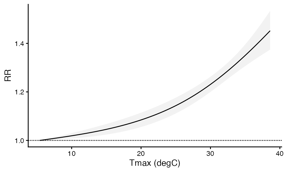
Finally, do some basic checks of the math using other utility functions to estimate the dispersion parameters and the variance-covariance matrix. Both of these functions will be useful once we are no longer using R functions to estimate the model.
First to check the dispersion
dispersion <- calc_dispersion(y = boston_deaths_tbl$daily_deaths,
                X = cb,
                stratum_vector = boston_deaths_tbl$strata,
                beta = coef(m_sub))
dispersion
#> [1] 3.366306
Next to check vcov
vcov_beta <- calc_vcov(y = boston_deaths_tbl$daily_deaths,
                X = cb,
                stratum_vector = boston_deaths_tbl$strata,
                beta = coef(m_sub))

# update with the dipserion parameter
t1 <- vcov_beta * dispersion

# check against the original model's vcov
t2 <- vcov(m_sub)
attributes(t2) <- NULL
t2 <- matrix(t2, nrow = nrow(t1), ncol = ncol(t1))

# should be the same
all.equal(t1, t2, tolerance = 1e-8)
#> [1] TRUE
Basic DLNM (using cityClimateHealth functions in
R)
The functionality above is what is encapsulated in the
condPois_1stage function. This is one of the chief
innovations of this package. Starting from a messy exposure and outcome
dataset, we can quickly estimate heat-health impacts in 3 lines.
We have built-in defaults for argvar,
arglag, and maxlag for the investigation of
warm-season non-fatal health impacts associated with increases in
temperature. We don’t need to check the dispersion parameter here since
this is using gnm under the hood.
# create exposure matrix
exposure_columns <- list(
  "date" = "date",
  "exposure" = "tmax_C",
  "geo_unit" = "TOWN20",
  "geo_unit_grp" = "COUNTY20"
)
boston_exposure_mat <- make_exposure_matrix(boston_exposure, exposure_columns,
                                            time_subset = list(month = 5:9))
#> Warning in make_exposure_matrix(boston_exposure, exposure_columns, time_subset = list(month = 5:9)): check about any NA, some corrections for this later,
#>             but only in certain columns
#> strata dt_by = 'day', setting strata as geo_unit:yr:mn:dow

# create outcome table
outcome_columns <- list(
  "date" = "date",
  "outcome" = "daily_deaths",
  "factor" = 'age_grp',
  "factor" = 'sex',
  "geo_unit" = "TOWN20",
  "geo_unit_grp" = "COUNTY20"
)
boston_deaths_tbl <- make_outcome_table(boston_deaths,  outcome_columns,
                                        time_subset = list(month = 5:9))
#> > No factors to collapse to, using all data
#> > grp_level == FALSE, so using geo_unit as strata
#> Missing outcome values introduced by xgrid were set to 0;
#>             assumes that every time in the dataset should have an outcome value
#> strata dt_by = 'day', setting strata as geo_unit:yr:mn:dow

# run the model
m1 <- condPois_1stage(exposure_matrix = boston_exposure_mat,
                  outcomes_tbl = boston_deaths_tbl)
#>
#> crossbasis args:
#>
#> maxlag: 5
#>
#> argvar:
#> List of 2
#>  $ fun  : chr "ns"
#>  $ knots: Named num [1:2] 26.2 31.7
#>   ..- attr(*, "names")= chr [1:2] "50%" "90%"
#>
#> arglag:
#> List of 2
#>  $ fun  : chr "ns"
#>  $ knots: num [1:2] 0.878 2.095
#>
#> strata:
#> BOSTON:yr2010:mn05:dow07
#> strata_min: 0
#> Warning in condPois_1stage(exposure_matrix = boston_exposure_mat, outcomes_tbl = boston_deaths_tbl): Centering point is outside the range of exposures in geo-unit BOSTON: Cen = 5.40, x_b = (6.00, 39.00).
#>         This means your zones are across too large of an area, or if exposure is factor there could
#>         be too few events in this area, or
#>         there are differences in exposures so much that the bases are quite different. Try limiting the geo-units passed in to those that are more similar, manually setting a centering point that you know each geo-unit has, or changing your exposure variable.
And plot the relative risk
plot(m1)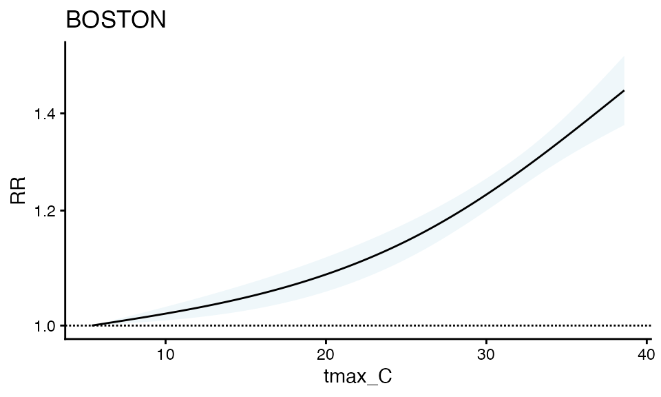
You can also get the RR table for your own usage
getRR(m1)
#>      tmax_C       RR     RRlb     RRub n_geo_names     model_class
#>       <num>    <num>    <num>    <num>      <char>          <char>
#>   1:    5.4 1.000000 1.000000 1.000000      BOSTON condPois_1stage
#>   2:    5.5 1.000395 1.000155 1.000636      BOSTON condPois_1stage
#>   3:    5.6 1.000791 1.000309 1.001272      BOSTON condPois_1stage
#>   4:    5.7 1.001186 1.000464 1.001909      BOSTON condPois_1stage
#>   5:    5.8 1.001582 1.000619 1.002546      BOSTON condPois_1stage
#>  ---
#> 329:   38.2 1.440253 1.367101 1.517320      BOSTON condPois_1stage
#> 330:   38.3 1.443200 1.368934 1.521494      BOSTON condPois_1stage
#> 331:   38.4 1.446152 1.370766 1.525684      BOSTON condPois_1stage
#> 332:   38.5 1.449111 1.372597 1.529891      BOSTON condPois_1stage
#> 333:   38.6 1.452077 1.374427 1.534113      BOSTON condPois_1stage
Multi-zone DLNM
You can also easily extend to a 1 stage multi-zone case. You don’t need to include population offset because within the geo_unit:year:month:dow strata the populations don’t change (one of the benefits of the conditional poisson setup – you would need to include a population offset if you were doing a time-series design).
# create exposure matrix
exposure_columns <- list(
  "date" = "date",
  "exposure" = "tmax_C",
  "geo_unit" = "TOWN20",
  "geo_unit_grp" = "COUNTY20"
)
middlesex_exposure <- subset(ma_exposure, COUNTY20 == 'MIDDLESEX')
middlesex_exposure_mat <- make_exposure_matrix(middlesex_exposure, exposure_columns,
                                               time_subset = list(month = 5:9))
#> Warning in make_exposure_matrix(middlesex_exposure, exposure_columns, time_subset = list(month = 5:9)): check about any NA, some corrections for this later,
#>             but only in certain columns
#> strata dt_by = 'day', setting strata as geo_unit:yr:mn:dow

# create outcome table
outcome_columns <- list(
  "date" = "date",
  "outcome" = "daily_deaths",
  "factor" = 'age_grp',
  "factor" = 'sex',
  "geo_unit" = "TOWN20",
  "geo_unit_grp" = "COUNTY20"
)
middlesex_deaths   <- subset(ma_deaths, COUNTY20 == 'MIDDLESEX')
middlesex_deaths_tbl <- make_outcome_table(middlesex_deaths,  outcome_columns,
                                           time_subset = list(month = 5:9))
#> > No factors to collapse to, using all data
#> > grp_level == FALSE, so using geo_unit as strata
#> Missing outcome values introduced by xgrid were set to 0;
#>             assumes that every time in the dataset should have an outcome value
#> strata dt_by = 'day', setting strata as geo_unit:yr:mn:dow

# run the model
m2 <- condPois_1stage(exposure_matrix = middlesex_exposure_mat,
                  outcomes_tbl = middlesex_deaths_tbl, multi_zone = TRUE,
                  global_cen = 15)
#>
#> crossbasis args:
#>
#> maxlag: 5
#>
#> argvar:
#> List of 2
#>  $ fun  : chr "ns"
#>  $ knots: Named num [1:2] 26 31.3
#>   ..- attr(*, "names")= chr [1:2] "50%" "90%"
#>
#> arglag:
#> List of 2
#>  $ fun  : chr "ns"
#>  $ knots: num [1:2] 0.878 2.095
#>
#> strata:
#> ACTON:yr2010:mn05:dow07
#> strata_min: 0
And plot - notice the tighter confidence interval
plot(m2)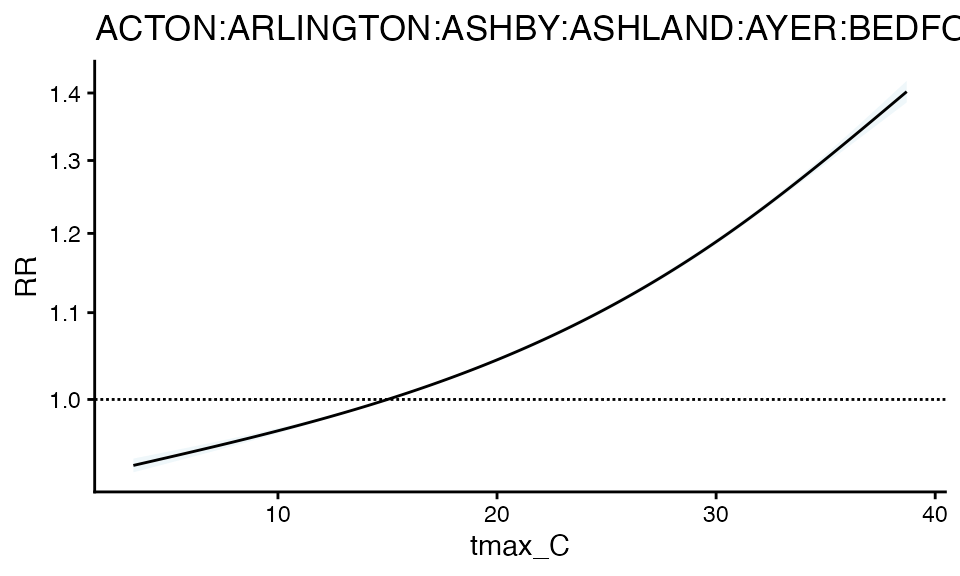
And get RR
getRR(m2)
#>      tmax_C        RR      RRlb      RRub                   n_geo_names
#>       <num>     <num>     <num>     <num>                        <char>
#>   1:    3.4 0.9301212 0.9231059 0.9371897 ACTON:ARLINGTON...(truncated)
#>   2:    3.5 0.9306360 0.9236853 0.9376389 ACTON:ARLINGTON...(truncated)
#>   3:    3.6 0.9311511 0.9242651 0.9380884 ACTON:ARLINGTON...(truncated)
#>   4:    3.7 0.9316666 0.9248454 0.9385382 ACTON:ARLINGTON...(truncated)
#>   5:    3.8 0.9321825 0.9254260 0.9389884 ACTON:ARLINGTON...(truncated)
#>  ---
#> 350:   38.3 1.3907853 1.3754494 1.4062922 ACTON:ARLINGTON...(truncated)
#> 351:   38.4 1.3936034 1.3779618 1.4094226 ACTON:ARLINGTON...(truncated)
#> 352:   38.5 1.3964278 1.3804785 1.4125612 ACTON:ARLINGTON...(truncated)
#> 353:   38.6 1.3992582 1.3829997 1.4157079 ACTON:ARLINGTON...(truncated)
#> 354:   38.7 1.4020947 1.3855253 1.4188624 ACTON:ARLINGTON...(truncated)
#>          model_class
#>               <char>
#>   1: condPois_1stage
#>   2: condPois_1stage
#>   3: condPois_1stage
#>   4: condPois_1stage
#>   5: condPois_1stage
#>  ---
#> 350: condPois_1stage
#> 351: condPois_1stage
#> 352: condPois_1stage
#> 353: condPois_1stage
#> 354: condPois_1stage
Multi-factor single beta coeff
you can also get it for factors
middlesex_deaths_tbl <- make_outcome_table(
  middlesex_deaths,  outcome_columns, time_subset = list(month = 5:9),
  collapse_to = 'age_grp')
#> > Factors in data
#> > grp_level == FALSE, so using geo_unit as strata
#> Missing outcome values introduced by xgrid were set to 0;
#>             assumes that every time in the dataset should have an outcome value
#> strata dt_by = 'day', setting strata as geo_unit:yr:mn:dow

# run the model
m3 <- condPois_1stage(exposure_matrix = middlesex_exposure_mat,
                  outcomes_tbl = middlesex_deaths_tbl,
                  global_cen = 15,
                  multi_zone = TRUE,
                  verbose = 1)
#> < age_grp : 0-17 >
#>
#> crossbasis args:
#>
#> maxlag: 5
#>
#> argvar:
#> List of 2
#>  $ fun  : chr "ns"
#>  $ knots: Named num [1:2] 26 31.3
#>   ..- attr(*, "names")= chr [1:2] "50%" "90%"
#>
#> arglag:
#> List of 2
#>  $ fun  : chr "ns"
#>  $ knots: num [1:2] 0.878 2.095
#>
#> strata:
#> ACTON:yr2010:mn05:dow07
#> strata_min: 0
#>
#> < age_grp : 18-64 >
#>
#> crossbasis args:
#>
#> maxlag: 5
#>
#> argvar:
#> List of 2
#>  $ fun  : chr "ns"
#>  $ knots: Named num [1:2] 26 31.3
#>   ..- attr(*, "names")= chr [1:2] "50%" "90%"
#>
#> arglag:
#> List of 2
#>  $ fun  : chr "ns"
#>  $ knots: num [1:2] 0.878 2.095
#>
#> strata:
#> ACTON:yr2010:mn05:dow07
#> strata_min: 0
#>
#> < age_grp : 65+ >
#>
#> crossbasis args:
#>
#> maxlag: 5
#>
#> argvar:
#> List of 2
#>  $ fun  : chr "ns"
#>  $ knots: Named num [1:2] 26 31.3
#>   ..- attr(*, "names")= chr [1:2] "50%" "90%"
#>
#> arglag:
#> List of 2
#>  $ fun  : chr "ns"
#>  $ knots: num [1:2] 0.878 2.095
#>
#> strata:
#> ACTON:yr2010:mn05:dow07
#> strata_min: 0

# plot
plot(m3)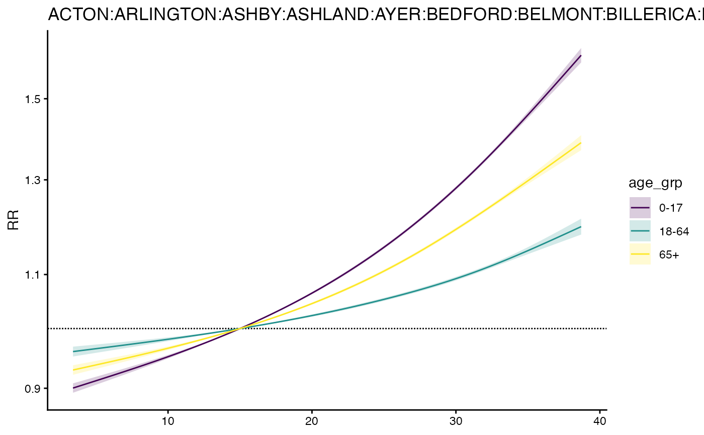
And get RR
getRR(m3)
#>       tmax_C age_grp        RR      RRlb      RRub          model_class
#>        <num>  <char>     <num>     <num>     <num>               <char>
#>    1:    3.4    0-17 0.9003521 0.8929348 0.9078311 condPois_1stage_list
#>    2:    3.5    0-17 0.9010769 0.8937259 0.9084883 condPois_1stage_list
#>    3:    3.6    0-17 0.9018023 0.8945178 0.9091461 condPois_1stage_list
#>    4:    3.7    0-17 0.9025284 0.8953105 0.9098045 condPois_1stage_list
#>    5:    3.8    0-17 0.9032552 0.8961040 0.9104636 condPois_1stage_list
#>   ---
#> 1058:   38.3     65+ 1.3780432 1.3611392 1.3951572 condPois_1stage_list
#> 1059:   38.4     65+ 1.3805675 1.3633300 1.3980230 condPois_1stage_list
#> 1060:   38.5     65+ 1.3830968 1.3655239 1.4008958 condPois_1stage_list
#> 1061:   38.6     65+ 1.3856309 1.3677209 1.4037754 condPois_1stage_list
#> 1062:   38.7     65+ 1.3881698 1.3699211 1.4066616 condPois_1stage_list
Changing the global_cen
You can change the global_cen and view the impact.
# run the model
m2 <- condPois_1stage(exposure_matrix = middlesex_exposure_mat, global_cen = 20, outcomes_tbl = middlesex_deaths_tbl, multi_zone = TRUE, verbose = 1)
#> < age_grp : 0-17 >
#>
#> crossbasis args:
#>
#> maxlag: 5
#>
#> argvar:
#> List of 2
#>  $ fun  : chr "ns"
#>  $ knots: Named num [1:2] 26 31.3
#>   ..- attr(*, "names")= chr [1:2] "50%" "90%"
#>
#> arglag:
#> List of 2
#>  $ fun  : chr "ns"
#>  $ knots: num [1:2] 0.878 2.095
#>
#> strata:
#> ACTON:yr2010:mn05:dow07
#> strata_min: 0
#>
#> < age_grp : 18-64 >
#>
#> crossbasis args:
#>
#> maxlag: 5
#>
#> argvar:
#> List of 2
#>  $ fun  : chr "ns"
#>  $ knots: Named num [1:2] 26 31.3
#>   ..- attr(*, "names")= chr [1:2] "50%" "90%"
#>
#> arglag:
#> List of 2
#>  $ fun  : chr "ns"
#>  $ knots: num [1:2] 0.878 2.095
#>
#> strata:
#> ACTON:yr2010:mn05:dow07
#> strata_min: 0
#>
#> < age_grp : 65+ >
#>
#> crossbasis args:
#>
#> maxlag: 5
#>
#> argvar:
#> List of 2
#>  $ fun  : chr "ns"
#>  $ knots: Named num [1:2] 26 31.3
#>   ..- attr(*, "names")= chr [1:2] "50%" "90%"
#>
#> arglag:
#> List of 2
#>  $ fun  : chr "ns"
#>  $ knots: num [1:2] 0.878 2.095
#>
#> strata:
#> ACTON:yr2010:mn05:dow07
#> strata_min: 0
plot(m2)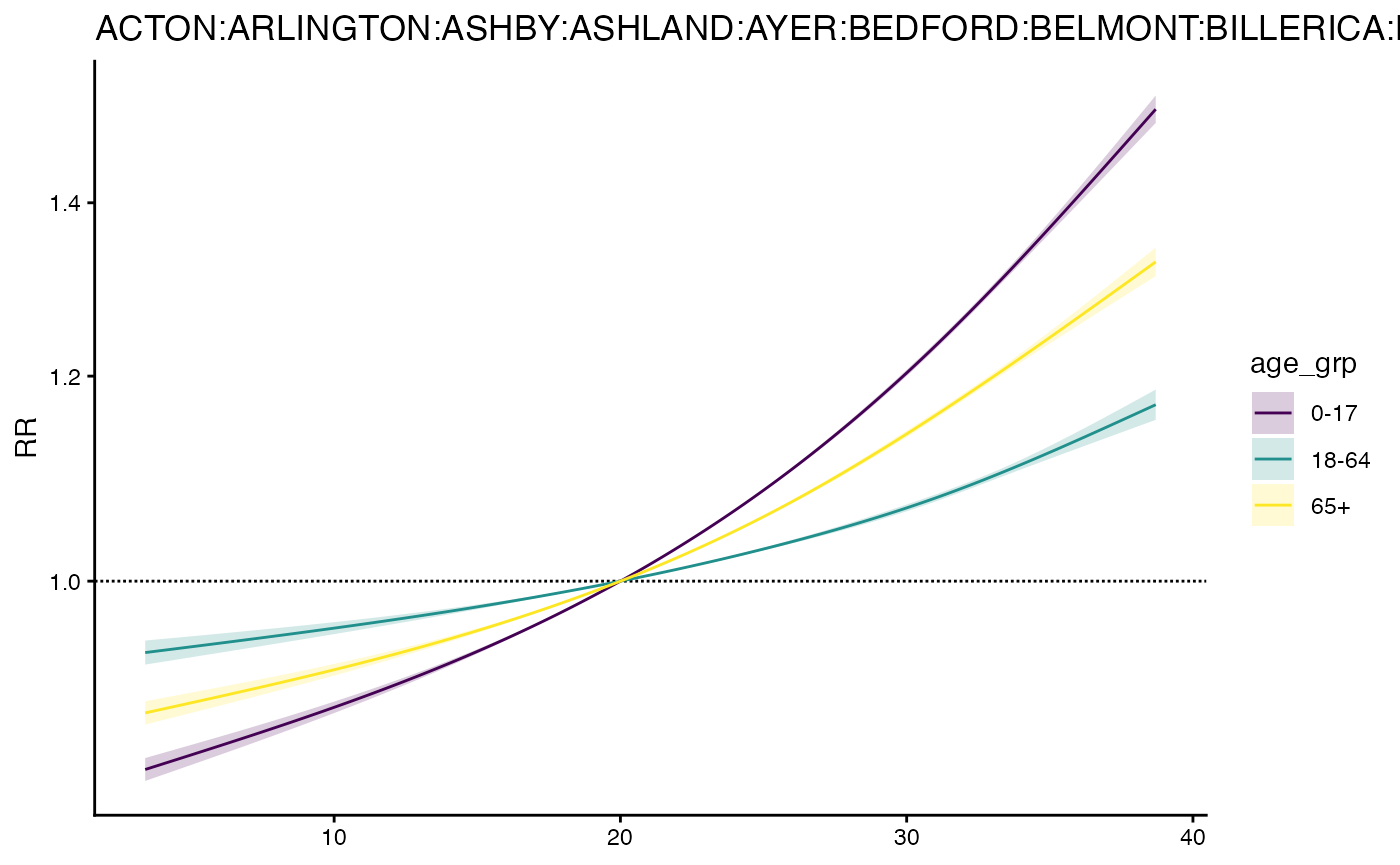
Note that global_cen must be within the range of exposures. Otherwise, the model is invalid and will not run.