Heat-Health Associations across multiple towns using `cityClimateHealth`
two_stage_demo.RmdWe can easily extend the functionality from
vignette("one_stage_demo") to estimate individual-zone
impacts across many zones.
Model
First create the inputs, using the same exposure_columns
and outcome_columns as before.
library(data.table)
exposure_columns <- list(
  "date" = "date",
  "exposure" = "tmax_C",
  "geo_unit" = "TOWN20",
  "geo_unit_grp" = "COUNTY20"
)

ma_exposure_matrix <- make_exposure_matrix(
  subset(ma_exposure,COUNTY20 %in% c('MIDDLESEX', 'WORCESTER')),
         exposure_columns,
  time_subset = list(
       month = 5:9,
       year = 2012:2015
     ))
#> Warning in make_exposure_matrix(subset(ma_exposure, COUNTY20 %in% c("MIDDLESEX", : check about any NA, some corrections for this later,
#>             but only in certain columns
#> strata dt_by = 'day', setting strata as geo_unit:yr:mn:dow

outcome_columns <- list(
  "date" = "date",
  "outcome" = "daily_deaths",
  "factor" = 'age_grp',
  "factor" = 'sex',
  "geo_unit" = "TOWN20",
  "geo_unit_grp" = "COUNTY20"
)
ma_outcomes_tbl <- make_outcome_table(
  subset(ma_deaths,COUNTY20 %in% c('MIDDLESEX', 'WORCESTER')),
  outcome_columns,
  time_subset = list(
       month = 5:9,
       year = 2012:2015
     ))
#> > No factors to collapse to, using all data
#> > grp_level == FALSE, so using geo_unit as strata
#> Missing outcome values introduced by xgrid were set to 0;
#>             assumes that every time in the dataset should have an outcome value
#> strata dt_by = 'day', setting strata as geo_unit:yr:mn:dow
Now run by using condPois_2stage. This does the Gasp
Extended2stage design in 1 function from these inputs and defaults for
argvar, arglag and maxlag.
Importantly, the estimates in each geo_unit are
bolstered by those in their geo_unit_grp by including a
random effect for geo_unit_grp in the mixmeta
model.
ma_model <- condPois_2stage(ma_exposure_matrix, ma_outcomes_tbl,
                            verbose = 1, global_cen = 10)
#> -- validation passed
#> -- stage 1
#>
#> crossbasis args:
#>
#> maxlag: 5
#>
#> argvar:
#> List of 2
#>  $ fun  : chr "ns"
#>  $ knots: Named num [1:2] 25.7 31.4
#>   ..- attr(*, "names")= chr [1:2] "50%" "90%"
#>
#> arglag:
#> List of 2
#>  $ fun  : chr "ns"
#>  $ knots: num [1:2] 0.878 2.095
#>
#> strata:
#> ACTON:yr2012:mn05:dow03
#> strata_min: 0
#>
#>
#> -- mixmeta
#> formula: ~ 1 | COUNTY20/TOWN20
#> -- stage 2
You can still view the RR output from a single zone:
plot(ma_model, "CAMBRIDGE")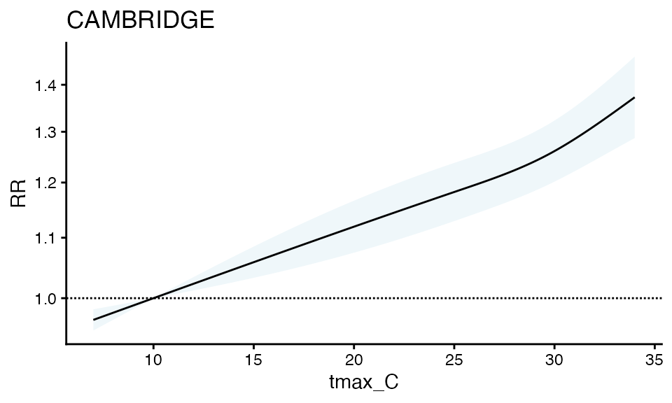 It does seem like this is a wider confidence interval than the solo
model – Perhaps this is expected given the variables around it? Worth
investigating in your dataset, as these are simulated data.
It does seem like this is a wider confidence interval than the solo
model – Perhaps this is expected given the variables around it? Worth
investigating in your dataset, as these are simulated data.
You can also plot by geo_unit_grp (TODO – a way to make
this cleaner to get to)
ma_model$`_`$grp_plt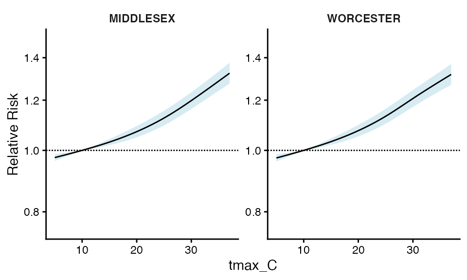
You can also make a forest plot at a specific exposure value
forest_plot(ma_model, 25.1)
#> Warning in forest_plot.condPois_2stage(ma_model, 25.1): plotting by group since
#> n_geos > 20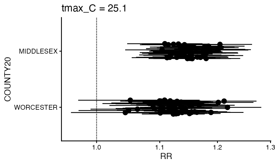
Finally you can also plot how the RR changes at specific expsoure
units across space – for this you need to bring in an sf
shapefile:
data("ma_towns")
ma_towns
#> Simple feature collection with 351 features and 36 fields
#> Geometry type: MULTIPOLYGON
#> Dimension:     XY
#> Bounding box:  xmin: 33863.75 ymin: 777634.4 xmax: 330838.8 ymax: 959743
#> Projected CRS: NAD83 / Massachusetts Mainland
#> # A tibble: 351 × 37
#>    STATEFP20 COUNTYFP20 COUSUBFP20 COUSUBNS20 GEOID20    NAMELSAD20       LSAD20
#>    <chr>     <chr>      <chr>      <chr>      <chr>      <chr>            <chr>
#>  1 25        003        34970      00618269   2500334970 Lenox town       43
#>  2 25        003        44385      00598751   2500344385 New Ashford town 43
#>  3 25        003        51580      00619422   2500351580 Otis town        43
#>  4 25        015        29265      00618202   2501529265 Hatfield town    43
#>  5 25        027        12715      00618359   2502712715 Charlton town    43
#>  6 25        011        05560      00619378   2501105560 Bernardston town 43
#>  7 25        003        59665      00619426   2500359665 Sandisfield town 43
#>  8 25        003        79985      00619430   2500379985 Williamstown to… 43
#>  9 25        017        31540      00618226   2501731540 Hudson town      43
#> 10 25        017        37875      00619404   2501737875 Malden city      25
#> # ℹ 341 more rows
#> # ℹ 30 more variables: CLASSFP20 <chr>, MTFCC20 <chr>, CNECTAFP20 <chr>,
#> #   NECTAFP20 <chr>, NCTADVFP20 <chr>, FUNCSTAT20 <chr>, ALAND20 <dbl>,
#> #   AWATER20 <dbl>, INTPTLAT20 <chr>, INTPTLON20 <chr>, TOWN20 <chr>,
#> #   TOWN_ID <int>, FIPS_STCO2 <dbl>, COUNTY20 <chr>, TYPE <chr>,
#> #   FOURCOLOR <int>, AREA_ACRES <dbl>, SQ_MILES <dbl>, POP1960 <dbl>,
#> #   POP1970 <dbl>, POP1980 <dbl>, POP1990 <dbl>, POP2000 <dbl>, …
head(ma_towns)
#> Simple feature collection with 6 features and 36 fields
#> Geometry type: MULTIPOLYGON
#> Dimension:     XY
#> Bounding box:  xmin: 48979.71 ymin: 869246.6 xmax: 166957.3 ymax: 942838.1
#> Projected CRS: NAD83 / Massachusetts Mainland
#> # A tibble: 6 × 37
#>   STATEFP20 COUNTYFP20 COUSUBFP20 COUSUBNS20 GEOID20 NAMELSAD20 LSAD20 CLASSFP20
#>   <chr>     <chr>      <chr>      <chr>      <chr>   <chr>      <chr>  <chr>
#> 1 25        003        34970      00618269   250033… Lenox town 43     T1
#> 2 25        003        44385      00598751   250034… New Ashfo… 43     T1
#> 3 25        003        51580      00619422   250035… Otis town  43     T1
#> 4 25        015        29265      00618202   250152… Hatfield … 43     T1
#> 5 25        027        12715      00618359   250271… Charlton … 43     T1
#> 6 25        011        05560      00619378   250110… Bernardst… 43     T1
#> # ℹ 29 more variables: MTFCC20 <chr>, CNECTAFP20 <chr>, NECTAFP20 <chr>,
#> #   NCTADVFP20 <chr>, FUNCSTAT20 <chr>, ALAND20 <dbl>, AWATER20 <dbl>,
#> #   INTPTLAT20 <chr>, INTPTLON20 <chr>, TOWN20 <chr>, TOWN_ID <int>,
#> #   FIPS_STCO2 <dbl>, COUNTY20 <chr>, TYPE <chr>, FOURCOLOR <int>,
#> #   AREA_ACRES <dbl>, SQ_MILES <dbl>, POP1960 <dbl>, POP1970 <dbl>,
#> #   POP1980 <dbl>, POP1990 <dbl>, POP2000 <dbl>, POP2010 <dbl>, POP2020 <dbl>,
#> #   POPCH10_20 <dbl>, HOUSING20 <dbl>, SHAPE_AREA <dbl>, SHAPE_LEN <dbl>, …

spatial_plot(ma_model, shp = ma_towns, exposure_val = 25.1)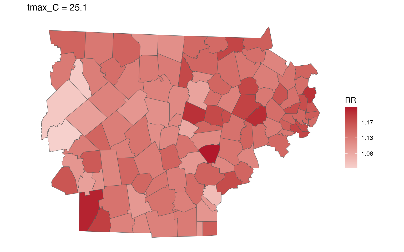
and You can get an RR table
getRR(ma_model)
#>           TOWN20  COUNTY20 tmax_C        RR      RRlb     RRub     model_class
#>           <char>    <char>  <num>     <num>     <num>    <num>          <char>
#>     1:     ACTON MIDDLESEX    7.0 0.9844671 0.9679222 1.001295 condPois_2stage
#>     2:     ACTON MIDDLESEX    7.1 0.9849752 0.9689752 1.001239 condPois_2stage
#>     3:     ACTON MIDDLESEX    7.2 0.9854837 0.9700294 1.001184 condPois_2stage
#>     4:     ACTON MIDDLESEX    7.3 0.9859924 0.9710848 1.001129 condPois_2stage
#>     5:     ACTON MIDDLESEX    7.4 0.9865016 0.9721413 1.001074 condPois_2stage
#>    ---
#> 32510: WORCESTER WORCESTER   33.6 1.2626515 1.1955548 1.333514 condPois_2stage
#> 32511: WORCESTER WORCESTER   33.7 1.2644009 1.1966017 1.336042 condPois_2stage
#> 32512: WORCESTER WORCESTER   33.8 1.2661529 1.1976434 1.338581 condPois_2stage
#> 32513: WORCESTER WORCESTER   33.9 1.2679074 1.1986804 1.341132 condPois_2stage
#> 32514: WORCESTER WORCESTER   34.0 1.2696643 1.1997131 1.343694 condPois_2stage
Model by factor
Only a small change is required to run the model by factor, e.g., age_grp:
ma_outcomes_tbl_fct <- make_outcome_table(
  subset(ma_deaths,COUNTY20 %in% c('MIDDLESEX', 'WORCESTER')),
  outcome_columns,
  time_subset = list(
       month = 5:9,
       year = 2012:2015
     ),
  collapse_to = 'age_grp')
#> > Factors in data
#> > grp_level == FALSE, so using geo_unit as strata
#> Missing outcome values introduced by xgrid were set to 0;
#>             assumes that every time in the dataset should have an outcome value
#> strata dt_by = 'day', setting strata as geo_unit:yr:mn:dow

head(ma_outcomes_tbl_fct)
#>          date TOWN20  COUNTY20 age_grp daily_deaths                  strata
#>        <IDat> <char>    <char>  <char>        <int>                  <char>
#> 1: 2012-05-01  ACTON MIDDLESEX    0-17           25 ACTON:yr2012:mn05:dow03
#> 2: 2012-05-01  ACTON MIDDLESEX   18-64           24 ACTON:yr2012:mn05:dow03
#> 3: 2012-05-01  ACTON MIDDLESEX     65+           24 ACTON:yr2012:mn05:dow03
#> 4: 2012-05-02  ACTON MIDDLESEX    0-17           26 ACTON:yr2012:mn05:dow04
#> 5: 2012-05-02  ACTON MIDDLESEX   18-64           26 ACTON:yr2012:mn05:dow04
#> 6: 2012-05-02  ACTON MIDDLESEX     65+           26 ACTON:yr2012:mn05:dow04
#>    strata_total     match_strata
#>           <int>           <char>
#> 1:          423 ACTON:2012-05-01
#> 2:          423 ACTON:2012-05-01
#> 3:          423 ACTON:2012-05-01
#> 4:          420 ACTON:2012-05-02
#> 5:          420 ACTON:2012-05-02
#> 6:          420 ACTON:2012-05-02
Run the model
ma_model_fct <- condPois_2stage(ma_exposure_matrix, ma_outcomes_tbl_fct,
                                verbose = 1, global_cen = 10)
#> < age_grp : 0-17 >
#> -- validation passed
#> -- stage 1
#>
#> crossbasis args:
#>
#> maxlag: 5
#>
#> argvar:
#> List of 2
#>  $ fun  : chr "ns"
#>  $ knots: Named num [1:2] 25.7 31.4
#>   ..- attr(*, "names")= chr [1:2] "50%" "90%"
#>
#> arglag:
#> List of 2
#>  $ fun  : chr "ns"
#>  $ knots: num [1:2] 0.878 2.095
#>
#> strata:
#> ACTON:yr2012:mn05:dow03
#> strata_min: 0
#>
#>
#> -- mixmeta
#> formula: ~ 1 | COUNTY20/TOWN20
#> -- stage 2
#>
#> < age_grp : 18-64 >
#> -- validation passed
#> -- stage 1
#>
#> crossbasis args:
#>
#> maxlag: 5
#>
#> argvar:
#> List of 2
#>  $ fun  : chr "ns"
#>  $ knots: Named num [1:2] 25.7 31.4
#>   ..- attr(*, "names")= chr [1:2] "50%" "90%"
#>
#> arglag:
#> List of 2
#>  $ fun  : chr "ns"
#>  $ knots: num [1:2] 0.878 2.095
#>
#> strata:
#> ACTON:yr2012:mn05:dow03
#> strata_min: 0
#>
#>
#> -- mixmeta
#> formula: ~ 1 | COUNTY20/TOWN20
#> -- stage 2
#>
#> < age_grp : 65+ >
#> -- validation passed
#> -- stage 1
#>
#> crossbasis args:
#>
#> maxlag: 5
#>
#> argvar:
#> List of 2
#>  $ fun  : chr "ns"
#>  $ knots: Named num [1:2] 25.7 31.4
#>   ..- attr(*, "names")= chr [1:2] "50%" "90%"
#>
#> arglag:
#> List of 2
#>  $ fun  : chr "ns"
#>  $ knots: num [1:2] 0.878 2.095
#>
#> strata:
#> ACTON:yr2012:mn05:dow03
#> strata_min: 0
#>
#>
#> -- mixmeta
#> formula: ~ 1 | COUNTY20/TOWN20
#> -- stage 2
And plot
plot(ma_model_fct, "CAMBRIDGE")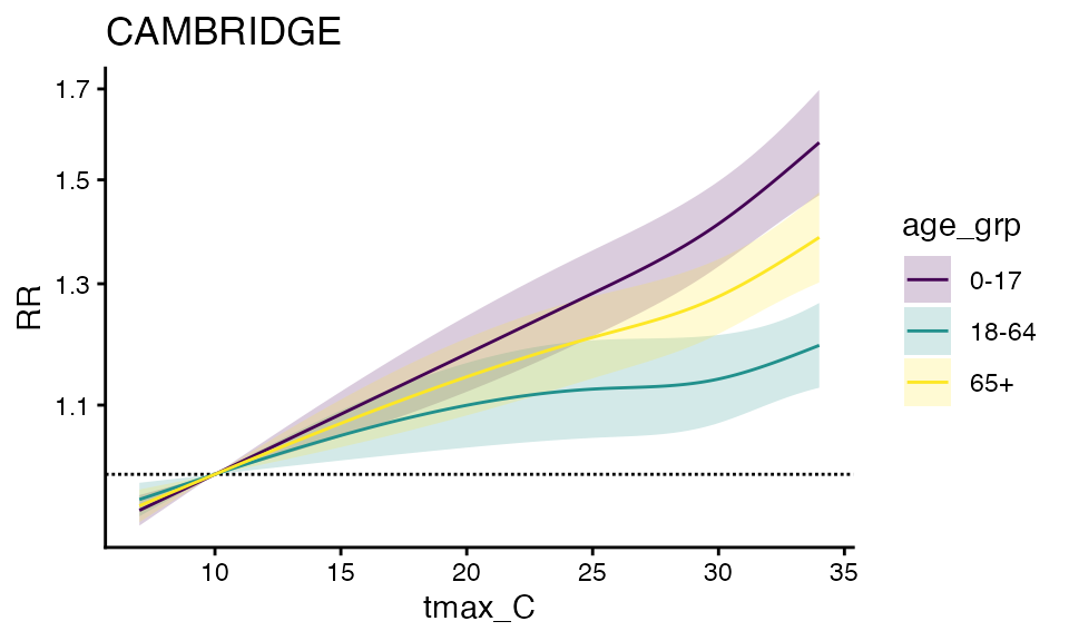
plot(ma_model_fct$`18-64`, "CAMBRIDGE", title = 'CAMBRIDGE: 18-64')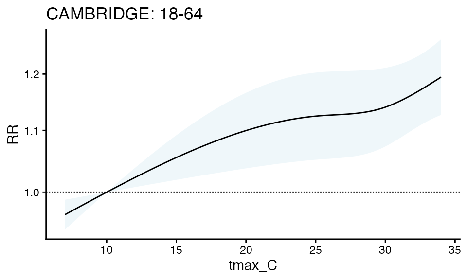
forest_plot(ma_model_fct, 25.1)
#> Warning in forest_plot.condPois_2stage_list(ma_model_fct, 25.1): plotting by
#> group since n_geos > 20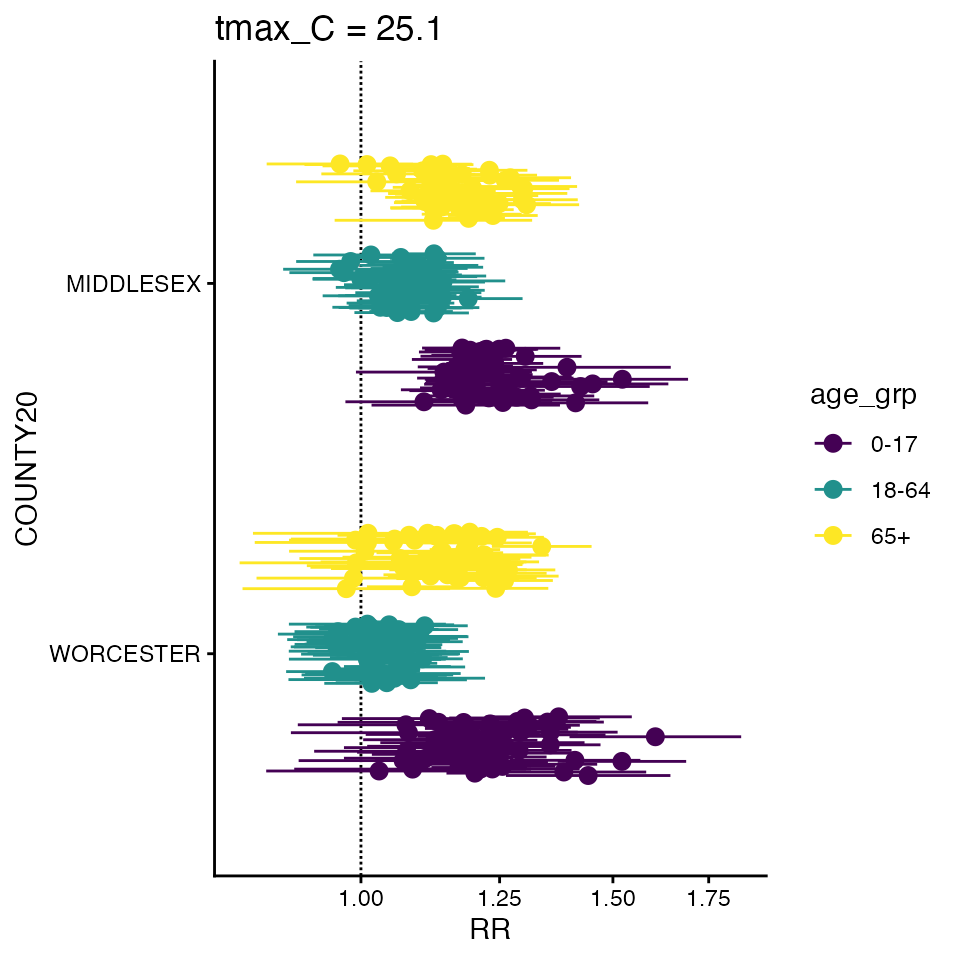
spatial_plot(ma_model_fct, shp = ma_towns, exposure_val = 25.1)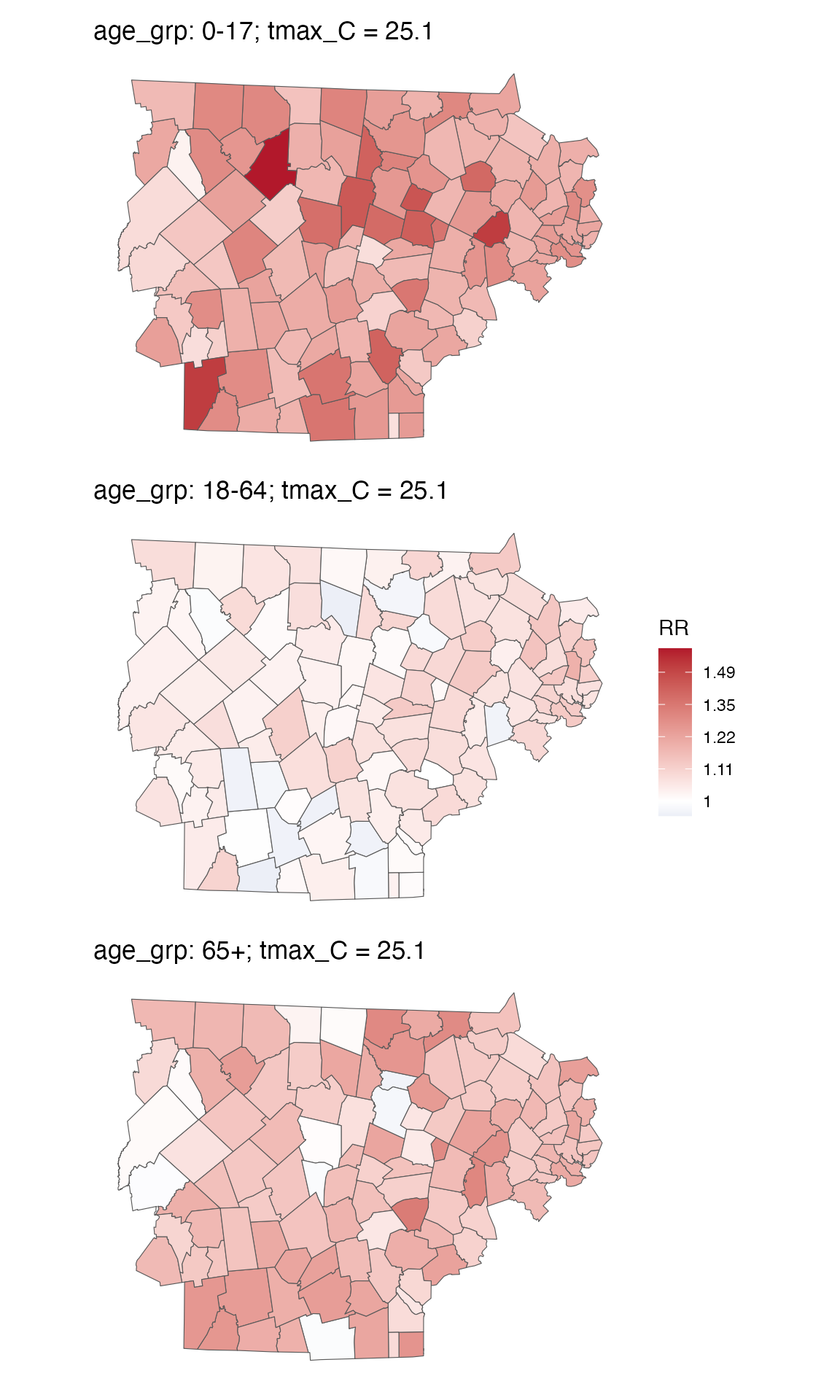 and You can get an RR table
getRR(ma_model_fct)
#>           TOWN20  COUNTY20 tmax_C        RR      RRlb     RRub age_grp
#>           <char>    <char>  <num>     <num>     <num>    <num>  <char>
#>     1:     ACTON MIDDLESEX    7.0 0.9791444 0.9572711 1.001518    0-17
#>     2:     ACTON MIDDLESEX    7.1 0.9798242 0.9586651 1.001450    0-17
#>     3:     ACTON MIDDLESEX    7.2 0.9805045 0.9600612 1.001383    0-17
#>     4:     ACTON MIDDLESEX    7.3 0.9811855 0.9614593 1.001316    0-17
#>     5:     ACTON MIDDLESEX    7.4 0.9818670 0.9628594 1.001250    0-17
#>    ---
#> 97538: WORCESTER WORCESTER   33.6 1.2671613 1.2062789 1.331117     65+
#> 97539: WORCESTER WORCESTER   33.7 1.2686961 1.2070137 1.333531     65+
#> 97540: WORCESTER WORCESTER   33.8 1.2702324 1.2077292 1.335970     65+
#> 97541: WORCESTER WORCESTER   33.9 1.2717706 1.2084263 1.338435     65+
#> 97542: WORCESTER WORCESTER   34.0 1.2733105 1.2091064 1.340924     65+
#>                 model_class
#>                      <char>
#>     1: condPois_2stage_list
#>     2: condPois_2stage_list
#>     3: condPois_2stage_list
#>     4: condPois_2stage_list
#>     5: condPois_2stage_list
#>    ---
#> 97538: condPois_2stage_list
#> 97539: condPois_2stage_list
#> 97540: condPois_2stage_list
#> 97541: condPois_2stage_list
#> 97542: condPois_2stage_list
Change the strata level
There may also be situations where you want to overwrite the strata to be a sub-strata level.
exposure_columns <- list(
"date" = "date",
"exposure" = "tmax_C",
"geo_unit" = "TOWN20",
"geo_unit_grp" = "COUNTY20"
)
ma_exposure_matrix <- make_exposure_matrix(
subset(ma_exposure, COUNTY20 %in% c('MIDDLESEX', 'WORCESTER', 'SUFFOLK') ), exposure_columns,
time_subset = list(
month = 5:9,
year = 2012:2015
),
grp_level = T, keep_unit_exposures = T)
#> Warning in make_exposure_matrix(subset(ma_exposure, COUNTY20 %in% c("MIDDLESEX", : check about any NA, some corrections for this later,
#> but only in certain columns
#> strata dt_by = 'day', setting strata as geo_unit:yr:mn:dow
outcome_columns <- list(
"date" = "date",
"outcome" = "daily_deaths",
"factor" = 'age_grp',
"factor" = 'sex',
"geo_unit" = "TOWN20",
"geo_unit_grp" = "COUNTY20"
)
ma_outcomes_tbl <- make_outcome_table(
subset(ma_deaths,COUNTY20 %in% c('MIDDLESEX', 'WORCESTER', 'SUFFOLK')), outcome_columns,
time_subset = list(
month = 5:9,
year = 2012:2015
),
grp_level = T, keep_unit_outcomes = T)
#> > No factors to collapse to, using all data
#> > grp_level == TRUE and keep_unit_outcomes == TRUE, so
#> keeping to geo_unit data but using geo_unit_grp as strata
#> Missing outcome values introduced by xgrid were set to 0;
#> assumes that every time in the dataset should have an outcome value
#> strata dt_by = 'day', setting strata as geo_unit:yr:mn:dow
ma_model <- condPois_2stage(ma_exposure_matrix,
ma_outcomes_tbl,
verbose = 2, global_cen = 10)
#> -- validation passed
#> -- stage 1
#> MIDDLESEX
#> crossbasis args:
#>
#> maxlag: 5
#>
#> argvar:
#> List of 2
#> $ fun : chr "ns"
#> $ knots: Named num [1:2] 25.6 30.7
#> ..- attr(*, "names")= chr [1:2] "50%" "90%"
#>
#> arglag:
#> List of 2
#> $ fun : chr "ns"
#> $ knots: num [1:2] 0.878 2.095
#>
#> strata:
#> ACTON:yr2012:mn05:dow03
#> strata_min: 0
#>
#> WORCESTER SUFFOLK
#> -- mixmeta
#> formula: ~ 1 | COUNTY20
#> IGLS iterations:
#> iter 0: value 6.693313e-12
#> converged
#> Newton iterations:
#> initial value -0.000000
#> iter 1 value 0.000000
#> final value -0.000000
#> converged
#> -- stage 2
#> MIDDLESEX WORCESTER SUFFOLK
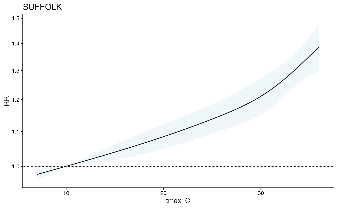
plot(ma_model, geo_unit = "SUFFOLK")