spatial_plot method for condPois_sb
spatial_plot.condPois_sb.Rdspatial_plot method for condPois_sb
Usage
# S3 method for class 'condPois_sb'
spatial_plot(x, shp, exposure_val, RRlimits = NULL, ...)
Arguments
- x
an object of class condPois_sb
- shp
an sf shapefile with an appropriate column at which to join
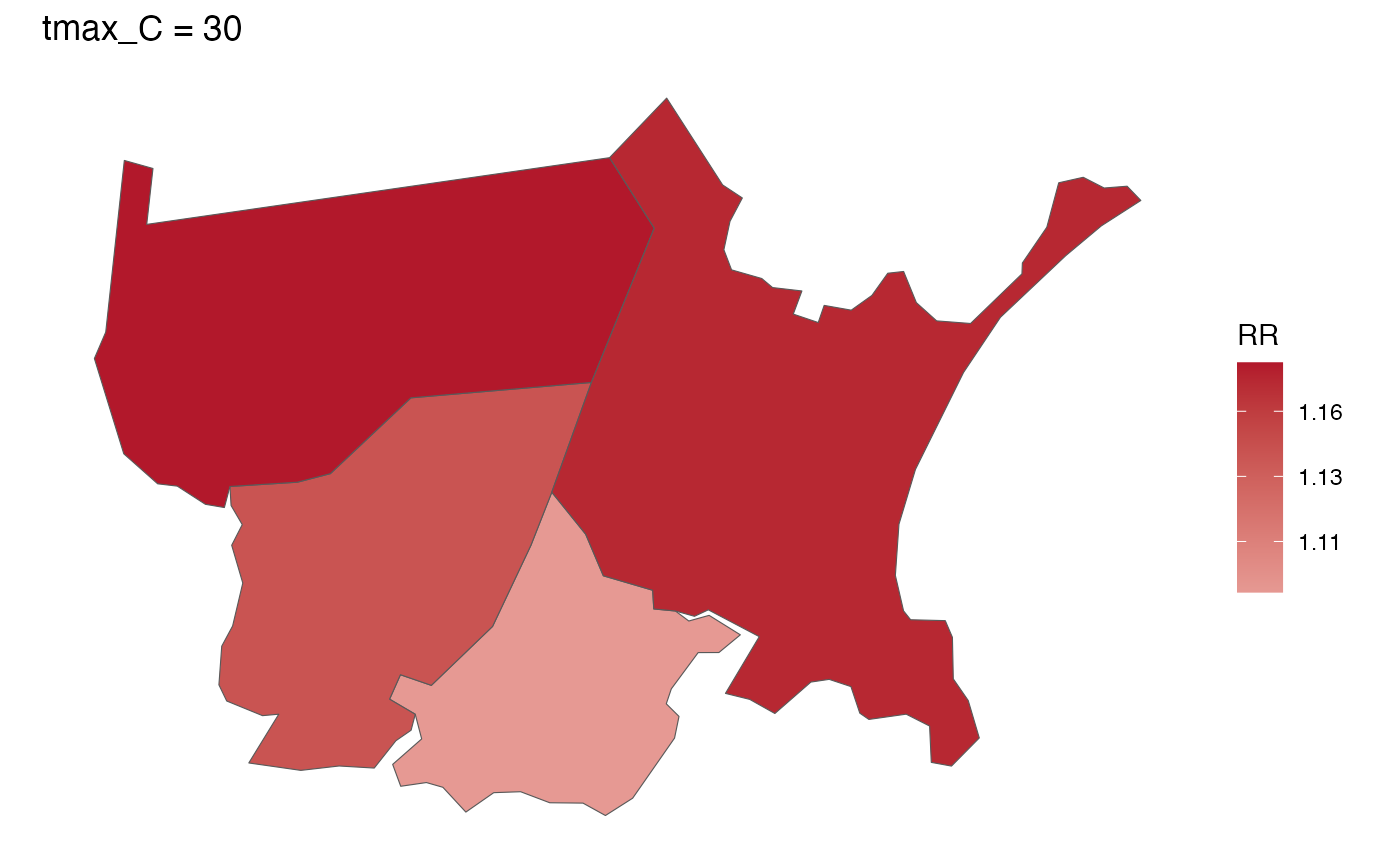
- exposure_val
exposure value at which to plot
- RRlimits
optional length-2 numeric vector of colour-scale limits for RR; defaults to the range of the plotted values
- ...
further arguments passed to or from other methods (currently unused)
Examples
towns <- c("CHELSEA", "EVERETT", "REVERE", "MALDEN")
exposure_columns <- list("date" = "date", "exposure" = "tmax_C",
                         "geo_unit" = "TOWN20", "geo_unit_grp" = "COUNTY20")
outcome_columns <- list("date" = "date", "outcome" = "daily_deaths",
                        "geo_unit" = "TOWN20", "geo_unit_grp" = "COUNTY20")
time_subset <- list(month = 5:9, year = 2012:2013)
exposure_mat <- make_exposure_matrix(subset(ma_exposure, TOWN20 %in% towns),
                                     exposure_columns, time_subset = time_subset)
#> -- NA values automatically removed
#> strata dt_by = 'day', setting strata as geo_unit:yr:mn:dow
outcomes_tbl <- make_outcome_table(subset(ma_deaths, TOWN20 %in% towns),
                                   outcome_columns, time_subset = time_subset)
#> Missing outcome values introduced by xgrid were set to 0;
#>             assumes that every time in the dataset should have an outcome value
#> strata dt_by = 'day', setting strata as geo_unit:yr:mn:dow
shp <- subset(ma_towns, TOWN20 %in% towns)
m <- condPois_sb(exposure_mat, outcomes_tbl, shp, global_cen = 20)
#>  STAN TYPE = laplace
#>  SPATIAL MODEL = bym2
#>
#> crossbasis args for geo_unit  CHELSEA :
#>
#> maxlag: 5
#>
#> argvar:
#> List of 2
#>  $ fun  : chr "ns"
#>  $ knots: Named num [1:2] 25.6 32.1
#>   ..- attr(*, "names")= chr [1:2] "50%" "90%"
#>
#> arglag:
#> List of 2
#>  $ fun  : chr "ns"
#>  $ knots: num [1:2] 0.878 2.095
#>
#> strata:
#> CHELSEA:yr2012:mn05:dow03
#> strata_min: 0
#>
#> min_n: 1
#>
#> truncate final RR and basis cen:  0
#> formula:
#>    daily_deaths ~ cb
#> family: quasipoisson
#> has to be one polygon per row in `shp`
#>  ...laplace optimize...
#> Initial log joint probability = -3358.51
#>     Iter      log prob        ||dx||      ||grad||       alpha      alpha0  # evals  Notes
#>       99      -3356.81     0.0025141       7.47411           1           1      127
#>     Iter      log prob        ||dx||      ||grad||       alpha      alpha0  # evals  Notes
#>      199       -3356.7    0.00032084      0.336854      0.2162           1      251
#>     Iter      log prob        ||dx||      ||grad||       alpha      alpha0  # evals  Notes
#>      211       -3356.7   0.000175631      0.220171      0.9493     0.09493      267
#> Optimization terminated normally:
#>   Convergence detected: relative gradient magnitude is below tolerance
#> Finished in  0.1 seconds.
#>  ...laplace sample...
#> Calculating Hessian
#> Calculating inverse of Cholesky factor
#> Generating draws
#> iteration: 0
#> iteration: 100
#> iteration: 200
#> iteration: 300
#> iteration: 400
#> iteration: 500
#> iteration: 600
#> iteration: 700
#> iteration: 800
#> iteration: 900
#> Finished in  0.4 seconds.
#>  ...laplace draws...
spatial_plot(m, shp = shp, exposure_val = 30)